Markov Chain Monte Carlo
|
Software |
|
Overview
A Markov Chain is a mathematical process that undergoes transitions from one state to another. Key properties of a Markov process are that it is random and that each step in the process is “memoryless;” in other words, the future state depends only on the current state of the process and not the past.
Description
A succession of these steps is a Markov chain.
This stochastic process may be described in terms of the conditional probability:

The possible values of Xi form the countable set S, which is the state space of the chain.
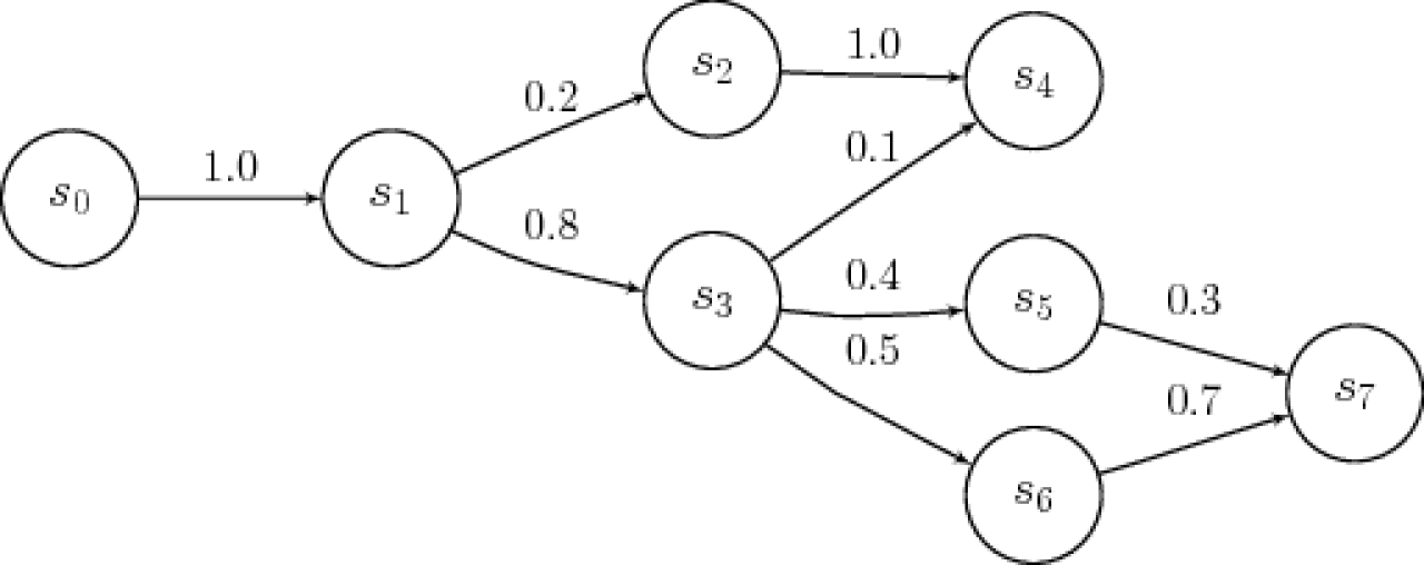
Markov chains are frequently seen represented by a directed graph (as opposed to our usual directed acyclic graph), where the edges are labeled with the probabilities of going from one state (S) to another.
A simple and often used example of a Markov chain is the board game “Chutes and Ladders.” The board consists of 100 numbered squares, with the objective being to land on square 100. The roll of the die determines how many squares the player will advance with equal probability of advancing from 1 to 6 squares. Each move is only determined the player’s present position. However, the board is filled with chutes, which move a player backward if landed on, and ladders, which will move a player forward. Once the stochastic Markov matrix, used to describe the probability of transition from state to state, is defined, there are several languages such as R, SAS, Python or MatLab that will compute such parameters as the expected length of the game and median number of rolls to land on square 100 (39.6 moves and 32 rolls, respectively).


In Bayesian analysis we make inferences on unknown quantities of interest (which could be parameters in a model, missing data, or predictions) by combining prior beliefs about the quantities of interest and evidence contained in an observed set of data. This is unlike so-called “frequentist” beliefs, where a hypothesis is tested without being assigned a probability; it must either be true or false, accepted or rejected. A Bayesian model has two parts: a statistical model that describes the distribution of data, usually a likelihood function, and a prior distribution that describes the beliefs about the unknown quantities independent of the data. A posterior distribution is then derived from the “prior” and the likelihood function.
Markov Chain Monte Carlo (MCMC) simulations allow for parameter estimation such as means, variances, expected values, and exploration of the posterior distribution of Bayesian models.
To assess the properties of a “posterior”, many representative random values should be sampled from that distribution. A Monte Carlo process refers to a simulation that samples many random values from a posterior distribution of interest. The name supposedly derives from the musings of mathematician Stan Ulam on the successful outcome of a game of cards he was playing, and from the Monte Carlo Casino in Las Vegas.
A Metropolis Algorithm (named after Nicholas Metropolis, a poker buddy of Dr. Ulam) is a commonly used MCMC process. This algorithm produces a so-called “random walk,” where a distribution is repeatedly sampled in small steps; is independent of the move before, and so is memoryless. This process is then used, for example, to describe a distribution or to compute an expected value.
The following example of a Metropolis Algorithm is provided with permission of Dr. Charles Dimaggio, who himself gives credit to John K. Kruschke.
“A politician is campaigning in 7 districts, one adjacent to the other. She wants to spend time in each district, but due to financial constraints, would like to spend time in each district proportional to the number of likely voters in that district. The only information available is the number of voters in the district she is currently in, and in those that are directly adjacent to it on either side. Each day, she must decide whether to campaign in the same district, move to the adjacent eastern district, or move to the adjacent western. On any given day, here’s how the decision is made whether to move or not:
-
Flip a coin. Heads to move east, tails to move west.
-
If the district indicated by the coin (east or west) has more voters than the present district, move there.
-
If the district indicated by the coin has fewer likely voters, make the decision based on a probability calculation:
-
calculate the probability of moving as the ratio of the number of likely voters in the proposed district, to the number of voters in the current district:
-
Pr[move] = voters in indicated district/voters in present district
-
Take a random sample between 0 and 1.
-
If the value of the random sample is between 0 and the probability of moving, move. Otherwise, stay put.
This “random walk” will, after many repeated sampling steps, be such that the time spent in each district is proportional to the number of voters in a district. Our Metropolis algorithm produced the following distribution:

-
At time=1, She is in district 4.
-
Flip a coin. The proposed move is to district 5.
-
Accept the proposed move because the voter population in district 5 is greater than that in district 4.
-
New day. Flip a coin. The proposed move is to district 6.Greater population, move.
-
New day. Flip a coin. The proposed move is to district7. Greater population, move.
-
At time=4, she is in district 7. Flip a coin. If the proposal is to move to district 6, base the decision to move on the probability criterion of 6/7. Draw a random sample between 0 and 1, if the value is between 0 and 6/7, move. Otherwise remain in district 7.
-
Perform this procedure many times.”
As it turns out, the actual target distribution of voters across the districts looks likes this:

What we see is that after many walks, the MCMC process “converges” to produce a distribution that is a mirror image of the actual distribution.
Of course, this is a highly simplified example, and MCMC algorithms can be created for continuous and multi-parameter distributions. This example does highlights several features of an MCMC process:
-
Burn-in: A random point was chosen to be the first sample. Note that in the distribution produced by the Metropolis algorithm, there is an increased density of samples around the starting district 4. It may take some time for the “walk” to move away from the initial starting point. If the target distribution has a sparser density in that region, the estimates produced from the MCMC will be biased. To mitigate this, an initial portion of a Markov chain sample is discarded so that the effect of initial values on inference is minimized. This is referred to as the “burn-in” period.
-
Efficiency: A probability density, or proposal distribution was assigned, to suggest a candidate for the next sample value, given the previous sample value. A typical choice, as in this example, is to let the proposal distribution be such that points closer to the previous sample point are more likely to be visited next. Whatever form (Gaussian or otherwise) the proposal distribution takes on, the goal is for this function to adequately and efficiently explore the sample space where the target distribution has the greatest density. If the target distribution is very broad and the proposal distribution is too “narrow,” it may take quite a while for the walk to find its way around the whole target distribution, and the MCMC will not be very efficient.
-
An acceptance ratio was used to decide whether to accept or reject the next proposed sample. Remember that this ratio was proportional to the density of the target distribution. If the proposal distribution is too broad, the acceptance ratio may infrequently be large enough to allow the walk to move from the current spot. The walk may then be trapped in a localized area of the target distribution.
There are many other sampling algorithms for MCMC. Another common technique is Gibb’s Sampling. Instead of choosing a candidate sample from a proposal distribution that represents the whole density, the Gibbs sample chooses a random value for a single parameter holding all the other parameters constant. This means that the target distribution and a proposal distribution do not need to be “tuned” for the walk to function efficiently.
CONVERGENCE:
When an MCMC has reached a stable set of samples from a stationary posterior distribution, it is said to have converged. Some models may never converge, or some of the reasons discussed above. For example, a poorly fit proposal distribution may lead to the walk never leaving a small area of the target distribution, or doing so very slowly. A high degree of autocorrelation between samples (some is expected) may also lead to very small steps in the walk, and slow or no convergence. Errors in programming and syntax have been cited by many authors as another reason for failure of convergence.
This is a perilous feature of MCMC algorithms: there is no one test or method to ensure that convergence has occurred. The danger is that the inferred posterior distribution may beabsolutely wrong, and parameter estimates will then also be incorrect. Therefore, it is considered a mandatory step in MCMC to asses for convergence. There are formal, but not definitive statistical tests of convergence. The Gelman-Rubin statistic assesses parallel chains with dispersed initial values to test whether they converge to the same target distribution. Examining trace plots of samples versus the simulation or iteration number is a simple way to visually test for convergence:

Excellent convergence, centered around a gamma of 3, with small fluctuations

Poor chain convergence
Applications:
Besides the important work of estimating the average length of a game of ‘Chutes and Ladders’, MCMC can also be used for epidemiological analyses where one would want to simulate a posterior distribution. The advantages to simulating a posterior distribution, is that if done correctly, one can estimate virtually all summaries of interest from the posterior distribution directly from the simulations. For example, one can estimate means, variances, and posterior intervals for a quantity of interest. One situation where this would be particularly advantageous is a setting where the observed data is incomplete; simulations to complete that data allow you to generate ‘true’ rather than ‘observed’ estimates. As example, Worby et al. use MCMC in their assessment of the effectiveness of isolation and decolonization measures to reduce MRSA transmission in hospital wards to account for imperfect and infrequent MRSA screening. Another situation where one might want to simulate a posterior distribution is when there is missing data in a survey. When the desired posterior distribution is intractable due to missingness in the observed data, the missing data can be simulated to create a tractable posterior distribution. MCMC procedures can be used where all missing data values are initially placed with plausible starting values. Then, based on certain parametric assumptions, a subsequent data value can be simulated based only on the previous value. Once this procedure is repeated, an iterative Markovian procedure is generated, which yields a successive simulation of the distribution of missing values, conditioned on both observed data and distributions of missing data previously simulated. These are just two examples of the many applications of MCMC methods. More examples are presented in example applications under the Articles subheading.
Readings
Textbooks & Chapters
Bayesian Methods: A Social and Behavioral Sciences Approach, Second Edition. Chapman & Hall/CRC, 2002, by Jeff Gill.
Doing Bayesian Data Analysis, 1st Edition. A Tutorial Introduction with R. Academic Press / Elsevier, 2011, by John K. Kruschke.
This text comes recommended by Dr. Charles DiMaggio; it is written for those who want to perform real -life analysis using Bayesian concepts and methods, including MCMC. It provides comprehensive R script, and bills itself as accessible to non-statisticians, with chapter 1.1 entitled: “Real People Can Read This Book.”
Markov Chain Monte Carlo: Stochastic Simulation for Bayesian Inference, Second Edition.London: Chapman & Hall/CRC, 2006, by Gamerman, D. and Lopes, H. F.
This book provides an introductory chapter on Markov Chain Monte Carlo techniques as well as a review of more in depth topics including a description of Gibbs Sampling and Metropolis Algorithm.
Monte Carlo Strategies in Scientific Computing. Springer-Verlag: New York., 2001, by J.S. Liu.
The fundamentals of Monte Carlo methods and theory are described. Strategies for conducting Markov Chain Monte Carlo analyses and methods for efficient sampling are discussed.
Monte Carlo Methods in Bayesian Computation, New York: Springer-Verlag, 2000, by Chen, M. H., Shao Q. M., and Ibrahim, J. G.
This book provides a thorough examination of Markov Chain Monte Carlo techniques. Sampling and Monte Carlo methods for estimation of posterior quantities are reviewed.
Markov Chain Monte Carlo in Practice. Chapman and Hall, 1996, W.R. Gilks, S. Richardson, D.J. Spiegelhalter (Eds.).
This book gives an overview of MCMC, as well as worked examples from several different epidemiological disciplines. The text goes into more depth than average student may need on the topic, and the programming has advanced since it was published in 1996.
Methodological Articles
A tutorial introduction to Bayesian inference for stochastic epidemic models using Markov chain Monte Carlo methods. O’Neill P., Mathematical Biosciences (2002) 180: 103–114.A good descriptive overview of MCMC methods for the use of modeling infectious disease outbreaks. Examples include: measles, influenza and smallpox.
Bayesian Modeling Using the MCMC Procedure. Chen F., SAS Global Forum 2009.
Comprehensive tutorial in the use of SAS for MCMC models, as well as a good overview of MCMC methods in general.
Markov Chain Monte Carlo in Practice: A Roundtable Discussion. Moderator: Robert Kass, Panelists Bradley Carlin, Andrew Gelman and Radford Neal. Edited discussion from the Joint Statistical Meetings in 1996.
A “nuts and bolts” discussion of the common applications, limitations, uses and misuses of MCMC methods. The first 3-4 pages offer a basic background on MCMC.
An Introduction to MCMC for Machine Learning. Andrieu C., De Freitas N., Doucet A., Jordan M, Machine Learning, (2003) 50: 5–43,
Despite the title, this article is a comprehensive lesson in the “main building blocks” of MCMC methods. It delves into the mathematical assumptions in detail and is quite technical. It is referenced as a background article by many other sources on MCMC.
Application Articles
Estimating the Effectiveness of Isolation and Decolonization Measures in Reducing Transmission of Methicillin-resistant Staphylococcus aureus in Hospital General Wards. Worby C., Jeyaratnam D., Robotham J., Kypraios T., O’Neill P., De Angelis D., French G., and Cooper B., Am. J. Epidemiol. Published online April 16th, 2013The utility of isolation and decolonization protocols on the spread of MRSA in a hospital setting is demonstrated using an MCMC algorithm to model transmission dynamics.
A Markov chain Monte Carlo algorithm for multiple imputation in large surveys. Schunk D., AStA (2008) 92: 101–114 Describes the use of MCMC in multiple imputation of missing data.
An MCMC algorithm for haplotype assembly from whole-genome sequence data. Bansal V., Halpern A., Axelrod N., Bafna V., Genome Res. (2008) 18: 1336-1346.
The authors create a novel MCMC algorithm to perform haplotype reconstruction/imputation.
Bayesian inference of hospital-acquired infectious diseases and control measures given imperfect surveillance data. Forrester M., Pettitt A., Biostatistics (2007) 8: .383–401
The authors use MCMC to model hospital MRSA transmission rates and and the probability of patient colonization on admission when missing data is present, a topic close to Jen Duchon’s heart. The reference section of this article is an excellent resource.
Decrypting Classical Cipher Text Using Markov Chain Monte Carlo. Chen J. and Rosenthal J., 2010
A cool use of MCMC: Code breaking! Priming the algorithm using different refence texts (War and Peace, Oliver Twist, a Wikipedia page on ice hockey), the authors use MCMC to break different kinds of ciphers.
A Bayesian model for cluster detection. Wakefield, J.; Kim, A. Biostatistics (2013), 14, 752–765.
Modelling life course blood pressure trajectories using Bayesian adaptive splines.
G Muniz-Terrera, E Bakra, R Hardy, FE Matthews, DJ Lunn. Statistical Methods in Medical Research (2014), Apr 25. [Epub ahead of print]
Another fun application: Some undergraduate students from the University of Wisconsin demonstrate the use of an MCMC analysis to find the expected length of a full game of “Chutes and Ladders.”
www.uwstout.edu/mscs/upload/Chutes-and-Ladders.ppt
Websites
-
Dr. Iain Murray from the University of Edinburg giving a lecture at the Machine Learning Summer School in 2009. This lecture is not geared toward epidemiologists or clinicians:http://videolectures.net/mlss09uk_murray_mcmc/
-
Simple, clear and intuitive discussion of MCMC on the “Stack Exchange” website. Found by posing the search “MCMC for dummies” to Google:http://stats.stackexchange.com/questions/165/how-would-you-explain-markov-chain-monte-carlo-mcmc-to-a-layperson
-
Dr. Simon Jackman’s work in Bayesian analysis for the Social sciences, including fairly complete lecture notes for his course by the same name can be found at: https://web.stanford.edu/class/polisci203/icpsr99.pdf
-
The R bloggers chime in on how long you’ll have to be sitting there with your 4 year old playing Chutes and Ladders. And how to figure out what square your kid was on if he has a meltdown and throws the pieces. Complete with R script! http://www.r-bloggers.com/basics-on-markov-chain-for-parents/
Courses
The International Society for Bayesian Analysis offers courses in general Bayesian statistical analysis. In past years, topics have included dedicated seminars on MCMC. Archived resources include videotaped lectures on MCMC methods (including Dr. Iain Murray’s – see below)
http://bayesian.org/
Monte Carlo Methods for Optimization
This graduate level course offered at the University of California, Los Angeles focuses on Monte Carlo methodology. Lecture notes are posted and available for review.
http://www.stat.ucla.edu/~sczhu/Courses/UCLA/Stat_202C/Stat_202C.html