Thin Plate Spline Regression

Overview

This page briefly describes thin plate splines and provides an annotated resource list.

Description

Thin plate splines are a type of smoothing spline used for the visualization of complex relationships between continuous predictors and response variables. Thin plate splines are ideal for examining the combined effect of two continuous predictors on a single outcome, because of their multi-dimensional appearance. Rather than a single curve, thin plate splines are represented as a bendable surface. Each continuous variable is plotted on an individual x-axis, creating a bivariate, two-dimensional surface. The outcome is then plotted on a y-axis, continuously across that bivariate surface in three-dimensions (Fig 1).

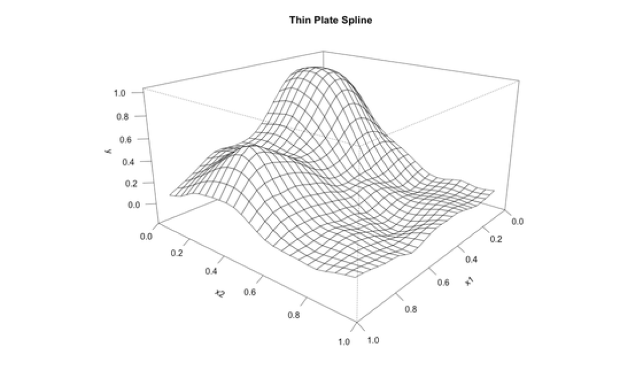
Fig. 1

Modeling Thin Plate Splines

Like other smoothing splines, thin plate splines are fitted using a generalized additive model (GAM), denoted by the equation:

g(E(Y)) = β0 + ƒ(X)+ λ

where β0 is a constant, ƒ(X) denotes a flexible function of x (or the sum of these functions for more than one x), and λ is the error term. The flexible function of x allows for the flexible fit of the predictor to the outcome that we are accustomed to seeing with splines, and the error term provides a “built-in” smoothing function based on a penalized least squares method. Increasing λ will increase the smoothness of the spline.

Thin plate splines receive their name from this built-in smoothing function. The error term (λ) can be described as the tension, or the amount of pressure, required to bend a “thin plate” of metal. The higher this tension, the more resistant the thin plate will be to bending – more resistant to the effects of X1 and X2 on Y – and the smoother the spline will appear. Figure 2 depicts the effect of increasing λ relative to the thin plate spline in figure 1, whereas figure 3 depicts a noisy version of the spline as a result of decreasing λ.

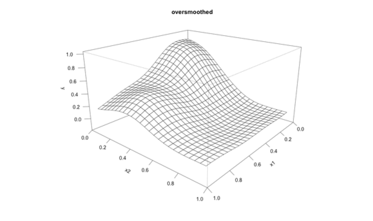
Fig. 2

Fig. 3(Figures 1 -3 from UW-Madison R Tutorial on Thin Plate Spline)

Advantages of Thin Plate Splines

The advantages to using thin plate splines, like other smoothing splines, is that GAMs do not require any a priori knowledge of the functional form of the data or the relationship of interest. The determination of node number and placement that can present a challenge in cubic splines, effectively becomes automated as part of the thin plate spline smoothing function. As the flexibility of GAMs is optimal in measuring the effect of continuous predictors, it similarly allows for optimal control of continuous confounders. The three-dimensional nature of thin plate splines makes them a powerful and attractive instrument for the visualization of complex predictor-response relationships. Heat maps may also be added to thin plate splines to further emphasize the curvature of the surface and create appealing visual graphics (Fig 4).

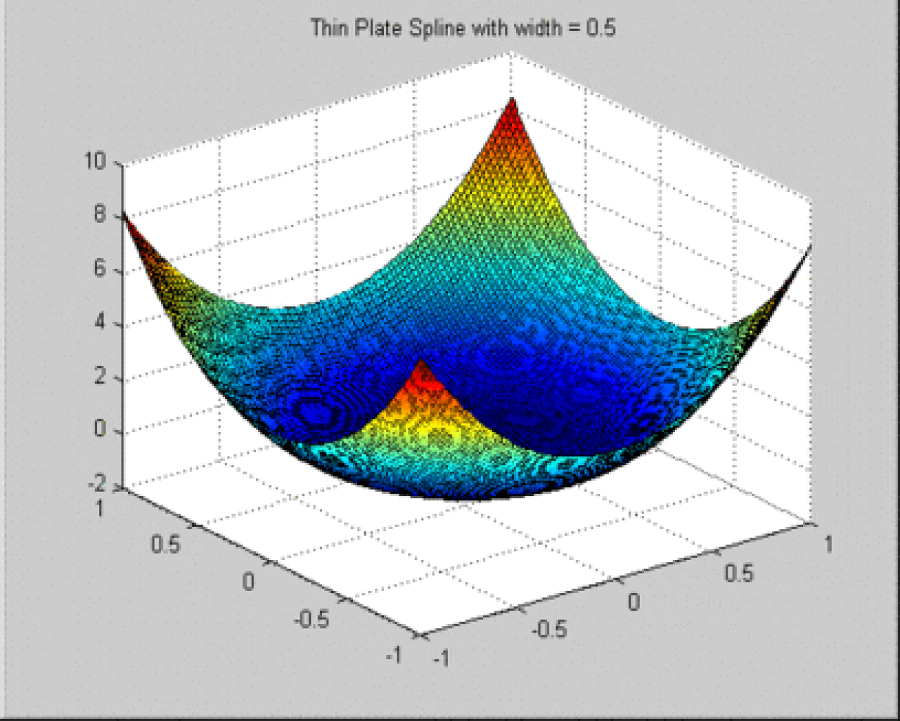
Fig. 4

Limitations of Thin Plate Splines

Just as complex data visualization is a key strength, it is also a limitation of using thin plate splines. The three-dimensionality of thin plate splines makes for the inclusion of confidence intervals difficult as the visual may become too complex for interpretation. Instead, upper and lower confidence intervals may each need to be plotted as separate thin plate splines and presented together with the “main effect” spline.

History and Uses

Thin plate splines were first used in 1970’s computer science in the subfield of computational geometry. The modeling approach is frequently used today in numerous fields, including engineering (e.g. structural design), anthropology (e.g. geometric morphometrics), ecology (e.g. population growth), and pattern recognition (e.g. fingerprint identification). Its common uses in health science research include the development and analysis of medical imaging techniques.

Thin Plate Splines in Epidemiology

Thin plate splines are historically less often used in epidemiological research, however the utility of thin plate splines in the field is clear and the increased use of this methodology should be more often considered. Access to powerful and open-source data visualization software such as R should make the use of thin plate splines a more feasible option for data analysis. See resource list below for example articles from the epidemiology literature.

Software Implementation

R can be used to fit a thin plate spline surface to irregularly spaced data. The smoothing parameter is chosen by generalized cross-validation. The assumed model is additive Y = f(X) +e where f(X) is a d dimensional surface. This function also works for just a single dimension and is a special case of a spatial process estimate (Kriging). A “fast” version of this function uses a compactly supported Wendland covariance and computes the estimate for a fixed smoothing parameter.

Tps(x, Y, m = NULL, p = NULL, scale.type = “range”, lon.lat = FALSE, miles = TRUE, …) fastTps(x, Y, m = NULL, p = NULL, theta, lon.lat=FALSE, …)

*See R help file on fields:tps for more information*

R can also be used to fit the specified generalized additive mixed model (GAMM) to data, by a call to lmerin the normal errors identity link case, or by a call to glmer otherwise (see lmer). Smoothness selection is by REML in the gaussian additive case and ML otherwise.
gamm4 is based on gamm from package mgcv, but uses lme4 rather than nlme as the underlying fitting engine via a trick due to Fabian Scheipl. gamm4 is more robust numerically than gamm, and by avoiding PQL gives better performance for binary and low mean count data. Its main disadvantage is that it can not handle most multi-penalty smooths (i.e. not te type tensor products or adaptive smooths) and there is no facilty for nlme style correlation structures. Tensor product smoothing is available via t2 terms.
For fitting generalized additive models without random effects, gamm4 is much slower than gam and has slightly worse MSE performance than gam with REML smoothness selection.
To use this function effectively it helps to be quite familiar with the use of gam and lmer.

gamm4(formula,random=NULL,family=gaussian(),data=list(),weights=NULL, subset=NULL,na.action,knots=NULL,…)

*See R help file on gamm4:gamm4 for more information*

Readings

Textbooks & Chapters

Chapter 19, Data Smoothing: Thin Plate Spline, SAS

Methodological Articles

S. N. Wood, Thin plate regression splines, J. R. Stat. Soc. Ser. B Stat. Methodol. 65, 95–114 (2003)

Lamina, C., Sturm, G., Kollerits, B., & Kronenberg, F. (2012). Visualizing interaction effects: A proposal for presentation and interpretation. Journal of Clinical Epidemiology, 65(8), 855-62. doi:http://dx.doi.org/10.1016/j.jclinepi.2012.02.013

Benedetti, A. and Abrahamowicz, M. (2004), Using generalized additive models to reduce residual confounding. Statist. Med., 23: 3781–3801. doi: 10.1002/sim.2073

Matuschek, H. Kliegl R. and Holschneider M. (2012) An Explicit ANOVA-like decomposition of Thin Plate Splines.
http://www.academia.edu/2616935/An_Explicit_ANOVA-like_decomposition_of_Thin_Plate_Splines

Marra, G., & Radice, R. (2010). Penalised regression splines: Theory and application to medical research. Statistical Methods in Medical Research, 19(2), 107-25. doi:http://dx.doi.org/10.1177/0962280208096688

Feng, CX. (2011) MODELS AND METHODS FOR SPATIAL DATA: APPLICATIONS IN EPIDEMIOLOGICAL, ENVIRONMENTAL AND ECOLOGICAL STUDIES Thesis. Department of Statistics and Actuarial Science, SIMON FRASER UNIVERSITY

Bookstein, Fred L., “Principal warps: thin-plate splines and the decomposition of deformations,”Pattern Analysis and Machine Intelligence, IEEE Transactions on , vol.11, no.6, pp.567,585, Jun 1989 doi: 10.1109/34.24792

Duchon, J. (1977) Splines minimizing rotation-invariant semi-norms in Solobev spaces. In Construction Theory of Functions of Several Variables. Berlin: Springer.

Application Articles

M. Stafoggia, J. Schwartz, F. Forastiere, and C. A. Perucci (2008). Does Temperature Modify the Association between Air Pollution and Mortality? A Multicity Case-Crossover Analysis in Italy. Am. J. Epidemiol. 167 (12): 1476-1485 first published online April 11, 2008 doi:10.1093/aje/kwn074

Jim Young, Patrick Graham, and Tony Blakely (2006). Modeling the Relation between Socioeconomic Status and Mortality in a Mixture of Majority and Minority Ethnic Groups. Am. J. Epidemiol. 164 (3): 282-291 first published online May 4, 2006 doi:10.1093/aje/kwj171

Kazembe LN, Mpeketula PMG (2010) Quantifying Spatial Disparities in Neonatal Mortality Using a Structured Additive Regression Model. PLoS ONE 5(6): e11180. doi: 10.1371/journal.pone.0011180

Anna Zajacova and Sarah A. Burgard (2012). Shape of the BMI-Mortality Association by Cause of Death, Using Generalized Additive Models: NHIS 1986–2006. J Aging Health. 24: 191-211, first published on May 10, 2011 doi:10.1177/0898264311406268

Courses

Lecture 11: Splines – Advanced Data Analysis, Carnegie Mellon University, Department of Statistics