Ridge Regression

Overview

This page briefly describes ridge regression and provides an annotated resource list.

Description

Defining the problem
The basic requirement to perform ordinary least squares regression (OLS) is that the inverse of the matrix X’X exists. X’X is typically scaled so that it represents a correlation matrix of all predictors. However, in certain situations (X’X)-1 may not be calculable. Specifically, if thedeterminant of X’X is equal to 0, then the inverse of X’X does not exist. In OLS, the parameter estimates depend on (X’X)-1, since they are estimated from the following equation:

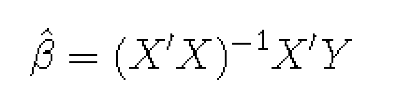
X’X represents a correlation matrix of all predictors; X represents a matrix of dimensions nxp, where n= # of observations and p= # of predictors in the regression model; Y represents a vector of outcomes that is length n; and X’ represents the transpose of X.

Thus, if the inverse of X’X cannot be calculated, the OLS coefficients are indeterminate. In other words, the parameter estimates will be highly unstable (i.e., they will have very high variances) and, consequently, will not be interpretable.

What causes (X’X)-1to be indeterminate?

• the number of parameters in the model exceeds the number of observations (n>p)

• multicollinearity

Diagnosing multicollinearity 
The easiest way to check for multicollinearity is to make a correlation matrix of all predictors and determine if any correlation coefficients are close to 1. However, this is somewhat subjective and does not provide information about the severity of multicollinearity.

Additional methods that are commonly used to gauge multicollinearity include:
1. Checking if at least one eigenvalue is close to 0.
2. Checking for large condition numbers (CNs). Commonly, the CN is calculated by taking the maximum eigenvalue and dividing it by the minimum eigenvalue: λmax/λmin. CN>5 indicates multicollinearity. CN>30 indicates severe multicollinearity.
3. Checking for high variance inflation factors (VIFs). The rule of thumb is that a VIF>10 indicates multicollinearity.

In SAS, VIFs can be obtained by using the code /vif.
In R, they can be calculated using the code vif() on a regression object. Importantly, this code requires the packages “car” and “HH”.

Options for dealing with multicollinearity
There are many ways to address multicollinearity, and each method has its benefits and disadvantages. Common methods include: variable selection, principal component regression, and ridge regression. Variable selection simply entails dropping predictors that are highly correlated with other predictors in the model. However, sometimes this is not feasible. For instance, a variable contributing to collinearity might be a main predictor of interest, a potential confounder, or a mediator, which needs to be adjusted for to measure the direct effect of a predictor on the outcome. Fortunately, both principal component regression and ridge regression allow retention of all explanatory variables of interest, even if they are highly collinear, and both methods return virtually identical results. However, ridge regression preserves the OLS interpretation of the regression parameters, while principal component regression does not. Thus, if the question of interest is “What is the relationship between eachpredictor in the model and the outcome?”, ridge regression may be more useful than principal component regression. Ridge regression also provides information regarding which coefficients are the most sensitive to multicollinearity.

Ridge regression
Ridge regression focuses on the X’X predictor correlation matrix that was discussed previously. Specifically, ridge regression modifies X’X such that its determinant does not equal 0; this ensures that (X’X)-1 is calculable. Modifying the matrix in this way effectively eliminates collinearity, leading to more precise, and therefore more interpretable, parameter estimates. But, in statistics, there is always a trade-off between variance and bias. Therefore, there is a cost to this decrease in variance: an increase in bias. However, the bias introduced by ridge regression is almost always toward the null. Thus, ridge regression is considered a “shrinkage method”, since it typically shrinks the beta coefficients toward 0.

How is X’X modified in ridge regression?
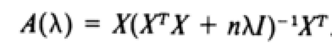
A ridge parameter, referred to as either λ or k in the literature, is introduced into the model. I will refer to this ridge parameter as k to avoid confusion with eigenvalues. The value of k determines how much the ridge parameters differ from the parameters obtained using OLS, and it can take on any value greater than or equal to 0. When k=0, this is equivalent to using OLS. The parameter k is incorporated into the following equation:

The above equation should look familiar, since it is equivalent to the OLS formula for estimating regression parameters except for the addition of kI to the X’X matrix. In this equation, I represents the identity matrix and k is the ridge parameter. Multiplying k by I and adding this product to X’X is equivalent to adding the value of k to the diagonal elements of X’X.

How does modifying X’X eliminate multicollinearity?
When there is multicollinearity, the columns of a correlation matrix are not independent of one another. This is a problem, because a matrix with non-independent columns has a determinant of 0. Therefore, the dependencies between columns must be broken so the inverse of X’X can be calculated. Adding a positive value k to the diagonal elements of X’X will break up any dependency between these columns. This will also cause the estimated regression coefficients to shrink toward the null; the higher the value of k, the greater the shrinkage. The intercept is the only coefficient that is not penalized in this way.

Choosing k
Hoerl and Kennard (1970) proved that there is always a value of k>0 such that the mean square error (MSE) is smaller than the MSE obtained using OLS. However, determining the ideal value of k is impossible, because it ultimately depends on the unknown parameters. Thus, the ideal value of k can only be estimated from the data.

There are many methods for estimating the ideal value of k. However, there is currently no consensus regarding which method is best.The traditional means of choosing k is the ridge trace plot which was introduced by Hoerl and Kennard (1970). This is a graphical means of selecting k. Estimated coefficients and VIFs are plotted against a range of specified values of k.
From this plot, Hoerl and Kennard suggest selecting the value of k that:

1. Stabilizes the system such that it reflects an orthogonal (i.e., statistically independent) system.

2. Leads to coefficients with reasonable values

3. Ensures that coefficients with improper signs at k=0 have switched to the proper sign

4. Ensures that the residual sum of squares is not inflated to an unreasonable value

However, these criteria are very subjective. Therefore, it is best to use another method in addition to the ridge trace plot. A more objective method is generalized cross validation (GCV). Cross validation simply entails looking at subsets of data and calculating the coefficient estimates for each subset of data, using the same value of k across subsets. This is then repeated multiple times with different values of k. The value of k that minimizes the differences in coefficient estimates across these data subsets is then selected. However, this is computationally intensive. GCV is just a weighted version of this method, and Golub et al (1979) have proven that the model with the smallest prediction errors can be obtained by simply selecting the value of k that minimizes the GCV equation shown below (note: Golub et al., 1979 refer to k as λ in their paper).

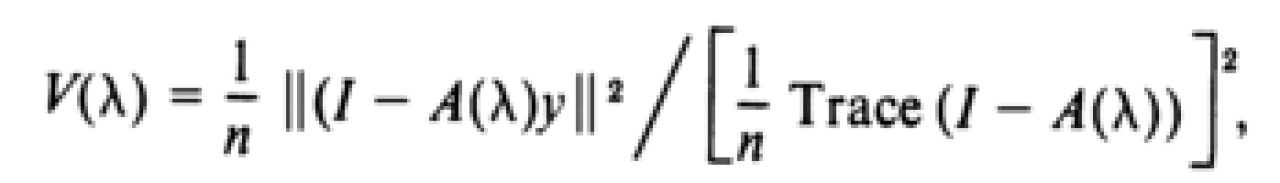
where

However, this need not be computed by hand. The value of k that minimizes this equation can be computed using R.

Example of how to implement ridge regression
Question of interest: Do arsenic metabolites have differential effects on blood glutathione concentrations?
Predictors of Interest: inorganic arsenic (InAs), monomethylarsenic (MMA), dimethylarsenic (DMA), measured in blood and log-transformed
Potential Confounders: age (log-transformed), sex, ever smoker (cig)
Outcome: glutathione measured in blood (bGSH)
Assessing multicollinearity:
proc reg data=fox;
model bGSH = ln_bInAs ln_bMMA ln_bDMA ln_age sex cig/vif;
run;

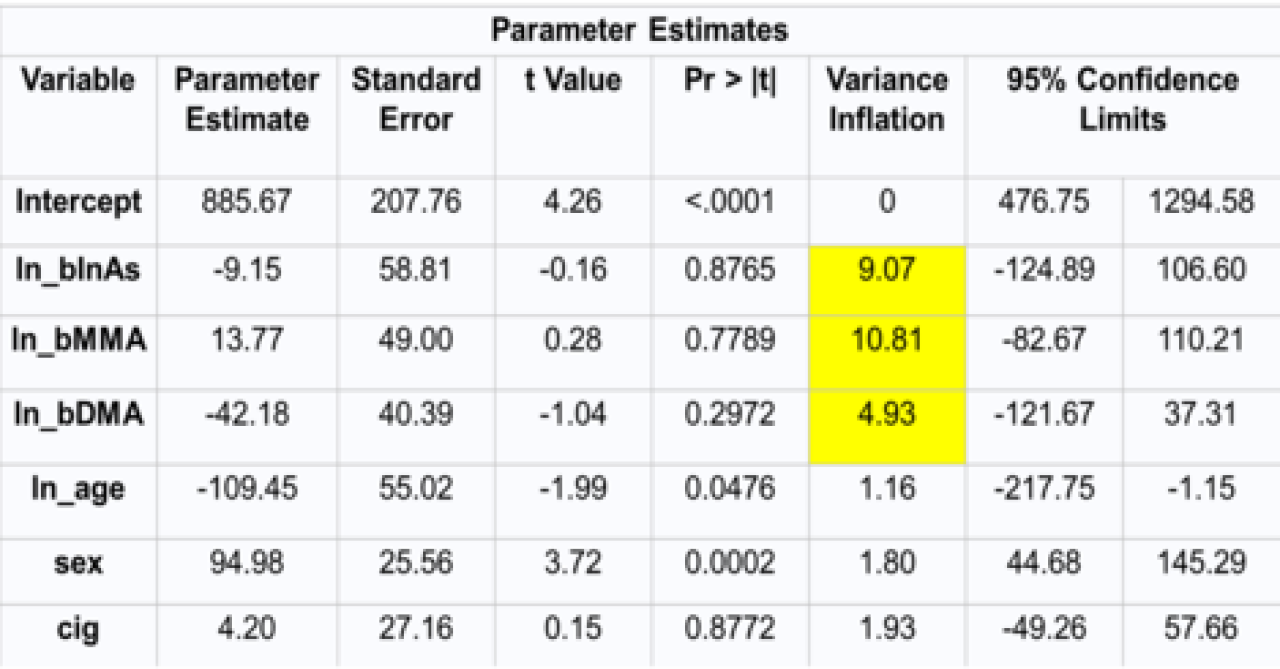
In this case, the VIFs are all very close to 10, so it may or may not be acceptable to use OLS. However, note how wide the confidence intervals are for the parameter estimates. Also, the parameter estimate for ln_bDMA is quite large. In environmental health studies, we rarely see such large coefficients. Ridge regression can therefore be used as a diagnostic tool in this situation to determine if these OLS estimates are reasonable.

Example Ridge Trace Plot in SAS:

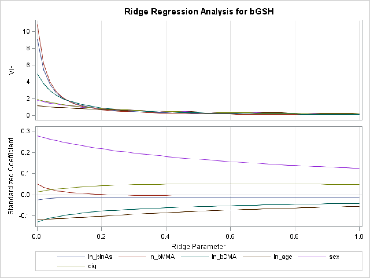
SAS ridge trace plots have two panels. The top panel shows the VIF for each predictor with increasing values of the ridge parameter (k). Each VIF should decrease toward 1 with increasing values of k, as multicollinearity is resolved. We see that in this case, the VIFs approach 1 when k is approximately 0.2.

The bottom panel shows the actual values of the ridge coefficients with increasing values of k. (SAS will automatically standardize these coefficients for you). At a certain value of k, these coefficients should stabilize (again, we see this occurring at values of k>0.2). Almost all of these parameters shrink toward the null with increasing values of k. Some parameter estimates may switch signs. Note that this is the case in my ridge trace plot for the variable ln_bMMA, shown in red. Using a k value of 0 (the OLS estimate), the association between ln_bMMA and bGSH is positive. However, once k is introduced into the model, and multicollinearity is resolved, one can see that the coefficient is actually negative (this switch in sign occurs at a k value of 0.24). This ridge trace plot therefore suggests that using OLS estimates might lead to incorrect conclusions regarding the association between this arsenic metabolite (blood MMA) and the outcome blood glutathione (bGSH).

I created the above plot using the following SAS Code:
proc reg data=fox outvif;
outest=fox_ridge ridge=0 to 1 by .02;
model bGSH=ln_bInAs ln_bMMA ln_bDMA ln_age sex cig;
run;

Note that “fox” is the name of my data set, “fox_ridge” is the name of a new data set that I am creating which will have the calculated ridge parameters for each value of k. You must specify your model and also the values of k you wish to look at. I examined all values of k between 0 and 1 by increments of 0.02, but note that these are small values of k to look at. Because the VIFs for my predictors were close to 10, the multicollinearity in this situation was not severe, so I did not need to examine large values of k.

You can also look at a table of all of your ridge coefficients and VIFs for each value of k by using the following statement:
proc print data=fox_ridge;
run;

Instructions for calculating GCV criteria in R:
1. Download the package ‘MASS’ so you can use the function lm.ridge()

2. Create a regression object using the lm.ridge() function. For example:
fox_ridge<-lm.ridge((bGSH~ln_bInAs + ln_bMMA + ln_bDMA + sex + cig + ln_age, lambda=seq(5,100,1))
##Note that I have specified a range of values for k (called “lambda” in R). GCV tends to select values of k close to 0, so it is best to restrict the possible range of k values.

3. Obtain GCV criterion for each value of k using the code $GCV following your regression object. For example:
fox_ridge$GCV

4. Select the value of k that yields the smallest GCV criterion

NOTE: SAS and R scale things differently. If you use the instructions I provided, which are specific to each program, you will get very similar ridge regression coefficients using either software. However, SAS and R will recommend different k values (due to the different scales), so you should not use the k value recommended in SAS to calculate ridge coefficients in R, nor should you use the k value recommended in R to calculate ridge coefficients in SAS.

Glossary:
Determinant: A value associated with a square matrix. Importantly, linear equations involving matrices only have unique solutions if the determinants of these matrices are not equal to 0.
Transpose: The transpose of a matrix A (e.g., A’) is simply matrix A with the values of the columns and rows switched. The row values of A are the column values of A’ and the column values of A are the row values of A’.
Indeterminate: A mathematical situation with more than one solution. If something is indeterminate, it cannot be precisely determined.
Eigenvalue: A number (λ) that, when multiplied by a non-zero vector (C), yields the product of C and a matrix (A). In other words, if a number
λ exists such that AC=λC, then λ is an eigenvalue.
Identity Matrix (also called the Unit Matrix): An nxn square matrix with values of 1 in the diagonal of the matrix and values of 0 in all other cells of the matrix. The identity matrix essentially serves as the value “1” in matrix operations. Examples of identity matrices are shown below:

2×2 Identity Matrix

3×3 Identity Matrix

4×4 Identity Matrix

Readings

Textbooks & Chapters

A useful resource for understanding regression in terms of linear algebra:
Appendix B (p.841-852) on “Matrices and Their Relationship to Regression Analysis” from Kleinbaum, Kupper, Nizam, and Muller. Applied Regression Analysis and Other Multivariable Methods. Belmont, CA: Thomson, 2008.

Chapter 8 from the following e-book is useful for understanding the problem of multicollinearity in terms of matrices and how ridge regression solves this problem:
Sections 8.1.5, 8.1.6 of http://sfb649.wiwi.hu-berlin.de/fedc_homepage/xplore/ebooks/html/csa/node171.html#SECTION025115000000000000000

For more detail…
Gruber, Marvin H.J. Improving Efficiency by Shrinkage: The James-Stein and Ridge Regression Estimators. New York: Marcel Dekker, Inc, 1998.

Methodological Articles

Hoerl AE and Kennard RW (2000). “Ridge Regression: Biased Estimation for Nonorthogonal Problems”. Technometrics;42(1):80.
Hoerl and Kennard (1968, 1970) wrote the original papers on ridge regression. In 2000, they published this more user-friendly and up-to-date paper on the topic.

Selecting K:
Golub GH, Heath M, Wahba G (1979). “Generalized Cross-Validation as a Method for Choosing a Good Ridge Parameter”. Technometrics;21(2):215-223. This is the go-to resource for understanding generalized cross-validation to select k, but it’s a bit abstruse, so see the resource listed under “Websites” for a simpler explanation.

Draper NR and van Nostrand CR (1979). “Ridge Regression and James-Stein Estimation: Review and Comments”.Technometrics;21(4):451-466. This paper offers a more critical take on ridge regression and describes the pros and cons of some of the different methods for selecting the ridge parameter.

Khalaf G and Shukur G (2005). “Choosing ridge parameter for regression problems”. Communications in Statistics –Theory and Methods; 34:1177-1182. This paper gives a nice and brief overview of ridge regression and also provides the results of a simulation comparing ridge regression to OLS and different methods for selecting k.

Commentary on Variable Selection vs. Shrinkage Methods:
Greenland S (2008). “Invited Commentary: Variable Selection versus Shrinkage in the Control of Multiple Confounders”. American Journal of Epidemiology; 167(5):523-529.

Application Articles

Holford TR, Zheng T, Mayne ST, et al (2000). “Joint effects of nine polychlorinates biphenyl (PCB) congeners on breast cancer risk”. Int J Epidemiol; 29:975-82.
This paper compares multiple methods for dealing with multicollinearity, including ridge regression.

Huang D, Guan P, Guo J, et al (2008). “Investigating the effects of climate variations on bacillary dysentery incidence in northeast China using ridge regression and hierarchical cluster analysis”. BMC Infectious Diseases;8:130.
This paper uses a combination of ridge regression and hierarchical cluster analysis to examine the influences of correlated climate variables on bacillary dysentery incidence.

Websites

Tutorials explaining basic matrix manipulations/linear algebra concepts:
https://www.khanacademy.org/math/linear-algebra/matrix_transformations

A nice web-site that explains cross-validation and generalized cross-validation in clearer language than the Golub article:
http://sfb649.wiwi.hu-berlin.de/fedc_homepage/xplore/ebooks/html/csa/node123.html

Courses

Courses:
Columbia has a course called Stat W4400 (Statistical Machine Learning), which briefly covers Ridge Regression (Lectures 13, 14). :
http://stat.columbia.edu/~cunningham/syllabi/STAT_W4400_2015spring_syllabus.pdf