Path Analysis
|
Websites |
|
Overview
Path analysis, a precursor to and subset of structural equation modeling, is a method to discern and assess the effects of a set of variables acting on a specified outcome via multiple causal pathways. Developed nearly a century ago by Sewall Wright, a geneticist working at the US Department of Agriculture, its early applications involved quantifying the contribution of genes vs. environment on traits such as guinea pig coloration and assessing whether temperature, humidity, radiation, or wind velocity had the greatest effect on transpiration in plants. Path analysis was slow to catch on in the world of biology, but in the second half of the 20th century found an avid following among social scientists and economists. Social and life course epidemiologists subsequently adopted the method as an effective way to distinguish direct from indirect effects and to test the strength of hypothesized patterns of causal relationships.
Description
Path analysis is based on a closed system of nested relationships among variables that are represented statistically by a series of structured linear regression equations. As such, path analysis is bound by the same set of assumptions as linear regression, as well as some additional restrictions that describe the allowable pattern of relations among variables. Variables are either exogenous, meaning their variance is not dependent on any other variable in the model, or endogenous, meaning their variance is determined by other variables in the model. Exogenous variables may or may not be correlated with other exogenous variables.
The pattern of relationships among variables is described by a path diagram, a type of directed graph. Variables are linked by straight arrows that indicate the directions of the causal relationships between them. Straight arrows may only point in one direction, as it is assumed that a variable cannot be both a cause and an effect of another variable; i.e., the model is recursive and there are no feedback loops. Curved, double-headed arrows indicate correlation between exogenous variables. Similar to DAGs, in path diagrams, causal “juice” can flow through arrows pointing in the same direction or pointing away from each other, but is blocked when two arrowheads meet. In addition to the arrows between variables in the model, there are arrows pointing toward each endogenous variable from points outside the model, indicating variance contributed by error and any unmeasured variables.
In figure 15.1, below, taken from Pedhazur’s Multiple Regression in Behavioral Research, variables 1 and 2 are exogenous and correlated, while variables 3, 4, and 5 are endogenous. The structural equation that would describe the relationship between variables 1 and 3 is:
r13 = p31 + p32*r12
where r is the correlation coefficient from a standard correlation matrix containing all of the variables in the model and the path coefficient p is the standardized beta coefficient from the linear regression model in which 1 and 2 are the independent variables and 3 is the dependent variable. (A note on notation: the first number in the path (or standardized beta) coefficient subscript represents the dependent variable (the head of the arrow) and the second number represents the independent variable (the tail of the arrow) in a causal relationship.) In general, a structural equation indicates that the total “juice,” or correlation between variables, is the sum of the “juice” that flows along each of the possible pathways that connect those two variables. In the example above, p31 is the proportion of the variance accounted for by the direct pathway between 1 and 3, while p32*r12 is the proportion of the variance accounted for by pathway that includes the segment between 1 and 2 and the segment between 2 and 3. The total variance along any particular pathway equals the product of the variance along the different segments of that pathway.
Similarly, the structural equation that would describe the relationship between variables 2 and 3 is:
r23 = p32 + p31*r12
and the series of structural equations that describe the contributions of variables 1, 2, and 3 to variable 4 (the coefficients of which come from the linear regression equation in which variable 4 is regressed on variables 1, 2, and 3) are:
r14 = p41 + p31*p43 + p42*r12 + p43*p32*r12
r24 = p42 + p32*p43 + p41*r12 + p43*p31*r12
r34 = p43 + p31*p41 + p32*p42 + p41*r12*p32 + p42*r12*p31
Notice that the number of structural equations (5) equals the number of parameters (p’s connecting variables) that need to be identified. This is called a just-identified model. The value of p3a is the square root of (1-r^2), using the unadjusted r-square value from the regression of 3 on variables 1 and 2, while the value of p4b is the square root of (1-r^2), using the unadjusted r-square value from the regression of 4 on variables 1, 2, and 3.
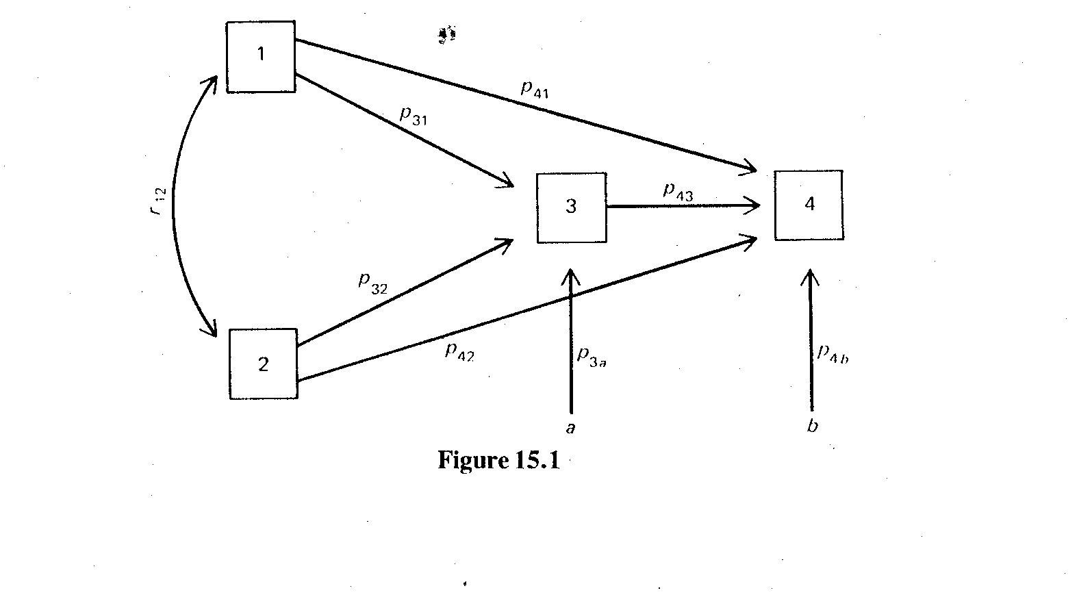
Once the path and correlation coefficients have been filled in, the utility of path analysis become clear. The total variance explained by each regression model can be partitioned, or “decomposed” into specific types of effects: direct, indirect, spurious (due to a common cause), and unanalyzed (because the directionality is unknown, as the path contributing to this effect includes a curved arrow). For example, in the equation for r14, p41 represents the direct effect, p31*p43 represents the indirect effect, and the remaining p42*r12 + p43*p32*r12 is unanalyzed. In the equation for r34 above, p43 represents the direct effect, while the entire remaining p31*p41 + p32*p42 + p41*r12*p32 + p42*r12*p31 is spurious; note that although they contain a curved arrow, the latter two pathways represent a common cause scenario.
Path analysis is always theory-driven; the same data can describe many different causal patterns, so it is essential to have an a priori idea of the causal relationships among the variables under consideration. That being said, path analysis can be used to refine a causal hypothesis. If, for example, a path coefficient is very small and the standardized beta is not statistically significant, it may make sense to eliminate that pathway. The new, “trimmed” model, which has the same number of variables but fewer pathways, can then be tested against the just-identified model (which becomes the null hypothesis) using any of several goodness-of-fit options. Failure to reject the null hypothesis indicates that the trimmed model still fits the data. In sum, path analysis may be used to test a causal model using data, but should not be used to develop a model from data.
While a path model may fit the data, beware–this does not mean that the causal hypothesis depicted in the path diagram has been validated. Some believe that the phrase “correlation does not imply causation” originated with Sewall Wright. Whether or not this is true, it is well remembered when performing path analysis. Although path diagrams are recursive, path models are based on correlations and cannot prove causation or even indicate the direction of a causal effect. Furthermore, those correlations are between variables in a given data set, so care must be taken before generalizing beyond the source population.
As mentioned above, path analysis is based on a number of assumptions:
-
Because path analysis involves the solution of multiple linear regression equations, the dependent variables for all equations must be approximately normally distributed and the relationships among the variables are assumed to be causal, linear and additive. Logistic regression equations, implying multiplicative relationships, cannot be substituted. Other curvilinear relations or interactions are also prohibited.
-
Residuals (a and b in the figure above) are not correlated with the variables that predict the outcome variables toward which they point. This means that a is not correlated with variables 1 and 2, and b is not correlated with variables 1, 2, and 3. This assumption implies that all relevant variables are included in the model, and any unmeasured variables are not correlated with the specified predictor variables.
-
Causation flows in one direction; there are no feedback loops.
-
The variables are measured without error.
-
Predictor variables may be continuous, ordinal categorical, or dichotomous, but there may be no dummy variables.
-
There is low multicollinearity among predictor variables in any of the linear regression equations.
In response to these limitations, structural equation modeling has evolved to allow for non-linear relations among variables, clustering, repeated measures, measurement error, feedback loops, and latent variables.
Readings
Textbooks & Chapters
Here’s a link to PDQ Statistics by Geoffrey R. Norman and David L. Streiner. Chapter 17 provides a readable introduction to path analysis and structural equation modeling:
https://vcarrion.people.uic.edu/pdq_stats.pdf
Chapter 15 of Elazar J. Pedhazur’s Multiple Regression in Behavioral Research gives a thorough presentation—with all the regression calculations done by hand!:
Pedhazur, Elazar J. Multiple Regression in Behavioral Research, 2nd ed. (Fort Worth, TX: Holt, Rinehart and Winston, Inc., 1982), p. 577-635.
A clear text which places path analysis in the context of causal inference:
Shipley, Bill. Cause and Correlation in Biology. (Cambridge, UK: Cambridge University Press, 2000).
Methodological Articles
Here are Sewall Wright’s original articles:
https://naldc.nal.usda.gov/download/IND43966364/PDF
https://www.gwern.net/docs/statistics/1934-wright.pdf
This is a more contemporary, excellent description of path analysis:
https://www.sciencedirect.com/science/article/pii/B0123693985004837
This is a nice simple summary:
http://core.ecu.edu/psyc/wuenschk/MV/SEM/Path.pdf
Application Articles
Gamborg, M., Andersen, P.K., Baker, J.L., Budtz-Jorgensen, E., Jorgensen, T., Jensen, G., Sorensen, T.I.A. (2009) Life course path analysis of birth weight, childhood growth, and adult systolic blood pressure. American Journal of Epidemiology, 169(10):1167-1178.
Check out this amazing example of a path diagram!
Wahlund, R. (1992). Tax changes and economic behavior: the case of tax evasion. Journal of Economic Psychology, 13:657-77.
Chemers, M. M., Hu, L.-T., and Garcia, B. F. (2001). Academic self-efficacy and first-year college student performance and adjustment. Journal of Educational Psychology, 93(1):55–64.
McLean, S.A., Paxton, S.J., Wertheim, E.H. (2013). Mediators of the relationship between media literacy and body dissatisfaction in early adolescent girls: implications for prevention. Body Image, March 5, e-pub ahead of print.
Leary, J.M., Lilly, C.L., Dino, G., Loprinzi, P.D., Cottrell, L. Parental influences in 7-9 year olds’ physical activity: a conceptual model. Preventive Medicine (2013), e-pub ahead of print.
Software
Path analysis in SAS using PROC CALIS:
https://stats.oarc.ucla.edu/sas/faq/how-can-i-do-path-analysis-in-sas/
Step-by-step description of how to do path analysis, including STATA and SPSS code:
http://www3.nd.edu/~rwilliam/stats2/l62.pdf
In R, you can do path analysis using several different packages: lavaan, ggm, OpenMx, plspm, and sem. Here’s a whole e-book on path modeling in R using the plspm package:
https://www.gastonsanchez.com/PLS_Path_Modeling_with_R.pdf
Courses
Short online SAS course from University of North Texas:
http://www.unt.edu/rss/class/Jon/SAS_SC/SAS_Module8_Path.htm