Least Absolute Shrinkage and Selection Operator (LASSO)
| Overview | Software |
| Description | Websites |
| Readings | Courses |
Overview
"Big Data" is a fuzzy concept but generally entails having a dataset that contains:
1. Numerous independent variables or predictors (denoted p) with p being large enough that investigators cannot put all the predictors into a model or may suspect that many of the variables are not associated with the outcome we are interested in predicting.
2. A large number of observations (denoted n) where n is large enough that the dataset can handle complex models.
In these scenarios investigators may be interested in the prediction of an outcome and finding a parsimonious subset of variables that are associated with that outcome. This is a hypothesis-generating approach to data analysis rather than a hypothesis-testing approach where statistical methods are used to determine the most predictive variables and build the model (rather than an investigator's theory). Penalized regression, especially the LASSO, can assist investigators interested in predicting an outcome by selecting the subset of the variables that minimizes prediction error.
Description
There are several other variable selection methods that have traditionally been used to build models, however their utility is more limited in the context of having a large p. For example:
1. Best Subset Selection: Involves testing each combination of variables and choosing the best model based on the set of variables that produces the best R2, AIC, BIC, AUC, Mean Square Error, etc. The number of models that have to be tested is 2p, which can be a computational burden as the number of predictors increases. For example, if p = 20, there are a total of 1,048,576 possible models that have to be compared.
2. Forward Step-wise Selection: Builds a prediction model by starting with an empty model and then adding variables one at a time, testing the improvement each variable adds to the model fit, and stopping the process once no additional variables involve the model's fit. The number of models that have to be tested is 1+p(p+1)/2. Thus if p = 20, then 211 models have to be compared.
3. Backward Step-wise Selection: Builds a prediction model by starting with a model with all variables included, then removing variables one at a time, testing the improvement of the removal of each variable to the model fit, and stopping the process once the removal of no additional variables improves the model's fit. The number of models that have to be tested is 1+p(p+1)/2. As with forward step-wise selection, if p = 20, then 211 models have to be compared.
While Forward and Backward Step-wise Selection are relatively efficient, they do not always fit the best model. For example, if Y is predicted with three variables X1, X2, and X3, where X1 is the single most predictive model, but X2 and X3 together is the best model, neither forward nor backward step-wise selection will choose that model.
Penalized regression can perform variable selection and prediction in a "Big Data" environment more effectively and efficiently than these other methods. The LASSO is based on minimizing Mean Squared Error, which is based on balancing the opposing factors of bias and variance to build the most predictive model.
Bias-Variance Trade-off
Definitions:
f (x) = True function relating X to Y
f (x) = Estimated function relating X to Y
Mean Squared Error = E{(Ynew – f(Xnew))2}
Mean square error is composed of three parts:
- Residual Variability or Error = E{(Ynew – f(Xnew))2}
- Squared Bias = E{(f(Xnew – E{f}(Xnew))2}
- Variance in f = E{(E{f}(Xnew) – f(Xnew))2}
Residual variation is the difference in expectation between the observed new Y values and the true function that relates the X to Y. This is the irreducible error that cannot be eliminated in statistical models. The squared bias is the difference between the true function relating X to Y and the function modeled using the data. Variance is the difference in the expectation of the function relating X to Y and the model estimated from the observed data and applied to the new X's.
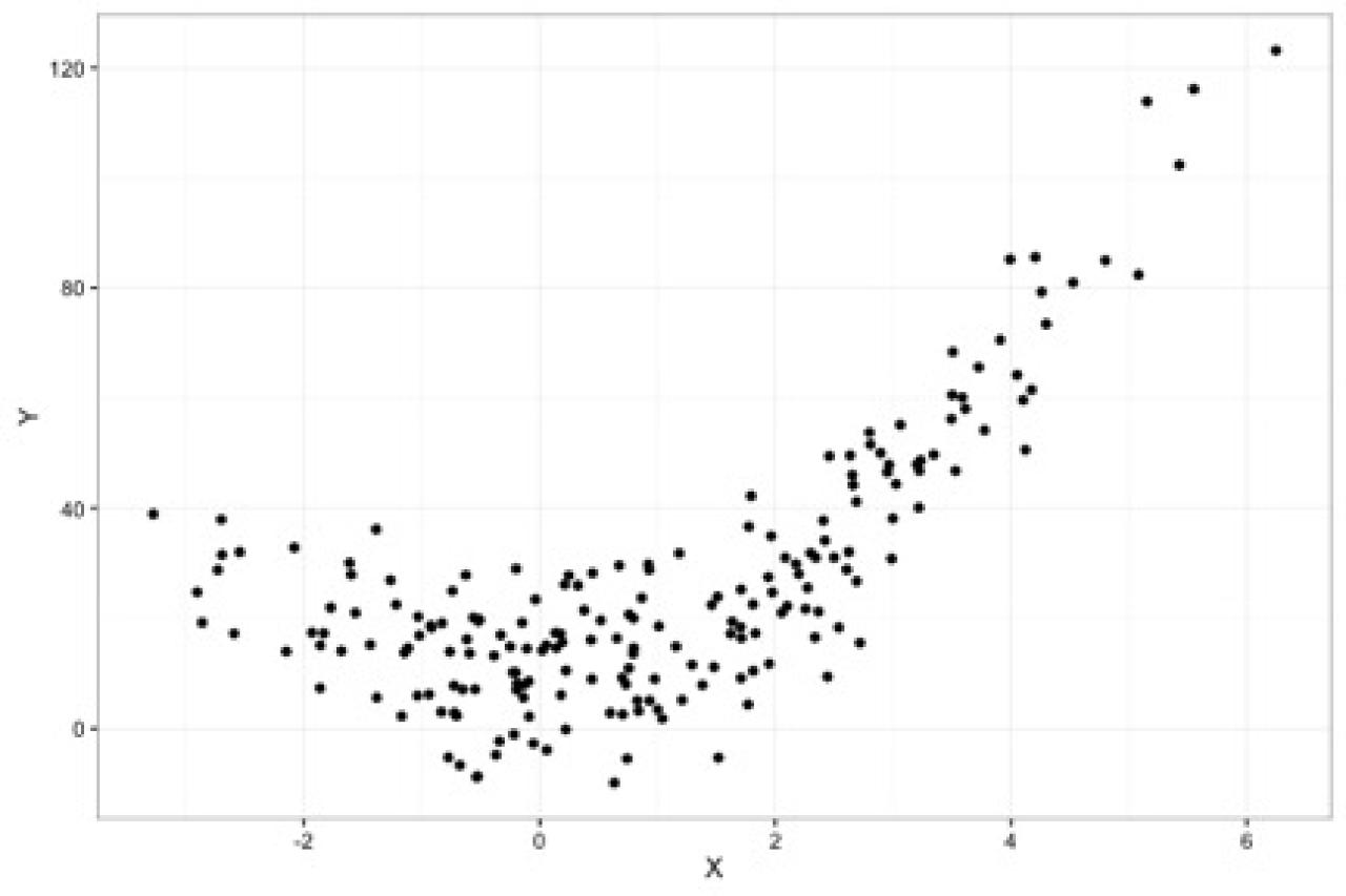
To give an example of the bias-variance trade-off, below is a dataset (N=200) where the true model relating X to Y is Y = 1.5*X + 3*X2 + error
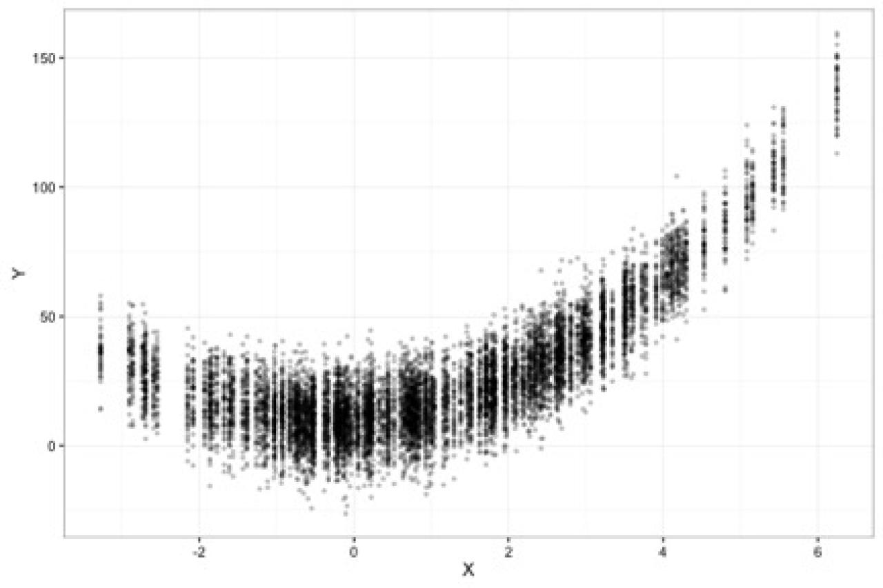
If we run the same study 50 times and plot all 50 studies in a single graph, the distribution of the X's will look like the below plot where the darker dots represent values of Y more likely to occur than the lighter grey values. The distribution of the observations is similar across the 50 studies, with random noise accounting for the differences across the 50 studies.
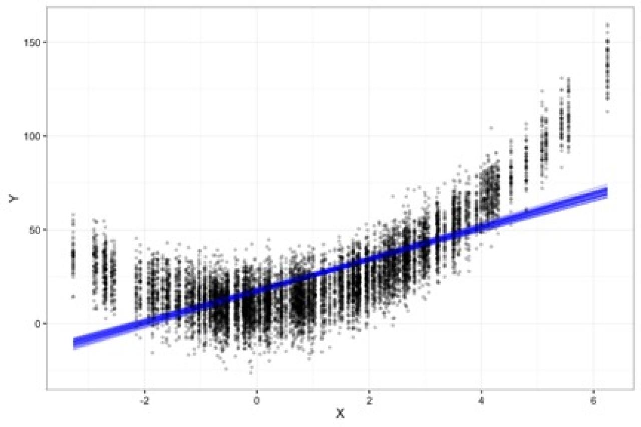
Squared Bias: If we fit the incorrect model, where Y = ß1*X without X2 term across all 50 studies and plot them together, the results would appear as below. The darker blue lines are where the model was estimated more often across the 50 studies. There is little variation between the studies, however the functional form of the model is incorrect, which means there is high squared bias. E.g., our estimated function relating X to Y is different from the true function.
Variance in f(x): If we fit the most complex model where for each X the value we predict for Y is the Y observed (i.e., our model contains 200 variables), then in each individual model, there is no bias but across the 50 studies there is significant variation in the function relating X to Y as seen in the plot below.

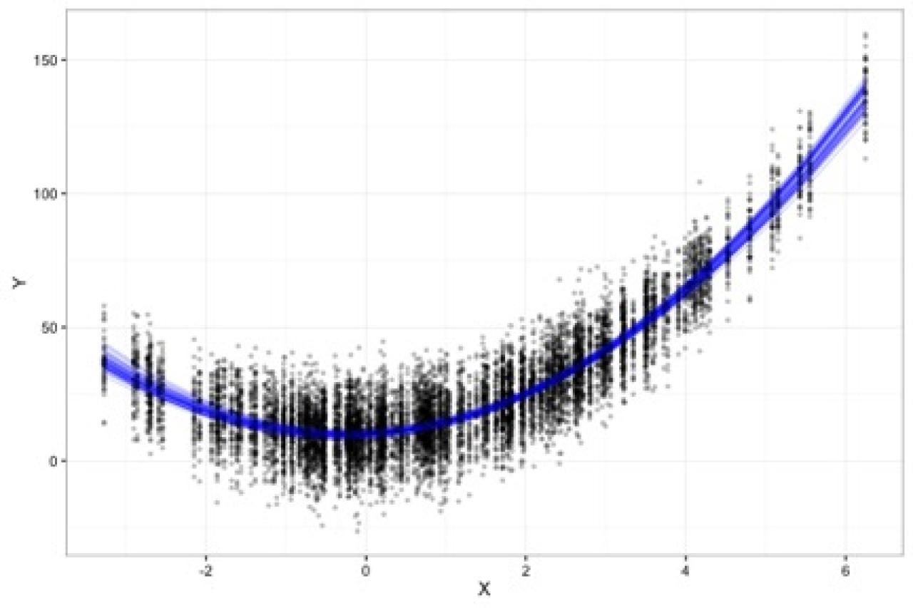
Residual Bias: If we fit the correct OLS model (e.g., Y = ß1*X + ß2*X2) across all 50 studies and plot them together on the same graph, the results would appear as below. There is little squared bias and little variation between the estimated functions. The only differences are the residual variation, which is the irreducible error, and is the spread of the observations around the blue line. The irreducible error is the difference between the observed Y and the true function relating X to Y.
The goal in model building is to select a model that minimizes both the squared bias and the variation. While a complex model will have little squared bias, it will have high variance. A model that is too sparse will have little variation across studies but high squared bias. The best fitting model will balance between bias and variance to have the lowest mean squared error.
The LASSO:
Ordinary Least Squares regression chooses the beta coefficients that minimize the residual sum of squares (RSS), which is the difference between the observed Y's and the estimated Y's.

The LASSO is an extension of OLS, which adds a penalty to the RSS equal to the sum of the absolute values of the non-intercept beta coefficients multiplied by parameter λ that slows or accelerates the penalty. E.g., if λ is less than 1, it slows the penalty and if it is above 1 it accelerates the penalty.

The LASSO can also be rewritten to be minimizing the RSS subject to the sum of the absolute values of the non-intercept beta coefficients being less than a constraint s. As s decreases toward 0, the beta coefficients shrink toward zero with the least associated beta coefficients decreasing all the way to 0 before the more strongly associated beta coefficients. As a result, numerous beta coefficients that are not strongly associated with the outcome are decreased to zero, which is equivalent to removing those variables from the model. In this way, the LASSO can be used as a variable selection method.

In order to find the optimal λ, a range of λ's are tested, with the optimal λ chosen using cross-validation. Cross-validation involves:
- Separating the data into a training set and a test set
- Building the model in the training set
- Estimating the outcome in the test set using the model from the training set
- Calculating MSE in the test set
One variant of cross-validation is the k-fold cross-validation where the data is separated into equal parts with each part serving as the test set for the model built in the training set. For example, in five-fold cross-validation, the data is split into 5 equal parts with the model built in 80% of the data and then tested in the remaining 20% of the data. Each part serves as the test set and the mean squared error is averaged across all the folds.

Scale Dependence: Continuous predictors should be mean centered and re-scaled to have equivalent standard deviations. This is necessary because the scale of the variable affects the size of the beta coefficient. For example, a beta coefficient for an income variable scaled in the thousands will be different than one for an unscaled income variable (e.g., an income of 55 versus 55,000). The beta coefficient for an income scaled in the thousands will be 1000 times the size of a beta coefficient for an unscaled variable. Since the LASSO shrinks coefficients, the unscaled coefficients will not be affected in the same way as the scaled coefficients and may lead to inefficient variables being included in the final model. Categorical variables should also be standardized, even though this affects the interpretation of the categorical variables.
Correlation among predictors: If several predictors are correlated, then the LASSO will choose only one of the predictors to be included in the model. The other correlated predictors will have their beta coefficients reduced to 0.
An example in R:
As an example, using the R package glmnet, first create three random explanatory variables (x1, x2, x3) that are mean centered at 0 with standard deviations of 1. An outcome variable, y, is created with the formula:
y = 2x1 + 7.1x2 – 3.4x3 + ε
set.seed (27572)
x1<-rnorm(n=20000)
set.seed(6827)
x2<-rnorm(n=20000)
set.seed(9327414)
x3<-rnorm(n=20000)
set.seed(6871673)
err<-rnorm(n=20000)
y<-2*x1+7.1*x2+3.4*x3+err
100 additional random variables are then added to the dataset that are completely unassociated with the outcome.
x<-cbind(x1, x2, x3)
seed<-3762
for(ii in 4:103){
ind<-ncol(x)+1
set.seed(seed)
new<-rnorm(n=nrow(x))
x<-cbind(x,new)
colnames(x)[ind]<-paste("x", ii, sep="")
seed+1
}
The function "cv.glmnet" implements cross-validation to find the λ that produces the most predictive model. The "cv.glmnet" requires the following inputs:
-
"x" is the matrix of predictors including any transformations you would like to include (e.g., x2, x3, etc.)
-
"y" is the continuous outcome you are interested in predicting
-
"alpha" is related to the elastic net, which both ridge regression and the LASSO are related to. For the purposes of this tutorial, alpha should equal 1, which indicates that LASSO regression should be performed.
-
nfolds is the number of k-folds cross-validation to run. Here we use 5-fold cross-validation though the default is 10-fold.
fit<-cv.glmnet(x=x,y=y, alpha=1, nfolds=5)
plot(fit)
The plot has the mean square error on the y-axis and the natural log of λ on the x-axis. Across the top is the number of variables included at these points. With a small lambda, three variables (x1, x2, and x3, the true predictive variables) are included. As λ increases, mean square error increases and eventually variables are dropped. The λ that results in the lowest mean square error is the dotted line closest to the y-axis. The second dotted line is the lambda that is within 1 standard error of the minimum. The authors of the LASSO recommend using the λ that is within one standard error of the minimum because it will often times lead to a more parsimonious model with fewer included variables and a minimal loss in mean squared error. The standard error in this case is the standard error of the averaged mean squared error for each λ.

In this example, the best λ was 0.03535056 and the λ one standard error above was 0.05128761. Using this value of λ, the estimated coefficients were close to the true coefficients that were used to create the y variable.
fit$lambda.min
## [1] 0.03535056
fit$lambda.1se
## [1] 0.05128761
c<-coef(fit,s='lambda.1se',exact=TRUE)
inds<-which(c!=0)
c[inds,]
## (Intercept) x1 x2 x3
## -0.007418572 1.954903924 7.035029531 3.359654825
Finally we can check the average cross-validated mean squared error when using the one standard error λ, which is 1.101439.
fit$cvm[which(fit$lambda==fit$lambda.1se)]
## [1] 1.014349
Readings
Textbooks:
James, G., Witten, D., Hastie, T., & Tibshirani, R. (2013). An introduction to statistical learning (Vol. 112). New York: springer.
Trevor J.. Hastie, Tibshirani, R. J., & Friedman, J. H. (2011). The elements of statistical learning: data mining, inference, and prediction. Springer.
Matignon, R. (2007). Data mining using SAS enterprise miner (Vol. 638). John Wiley & Sons.
Articles:
Tibshirani, R. (1996). Regression shrinkage and selection via the lasso. Journal of the Royal Statistical Society. Series B (Methodological), 267-288.
Tibshirani, R. (1997). The lasso method for variable selection in the Cox model. Statistics in medicine, 16(4), 385-395.
Software
Websites
https://cran.r-project.org/web/packages/glmnet/index.html
https://web.stanford.edu/~hastie/glmnet/glmnet_alpha.html
https://www.coursera.org/learn/predictive-analytics
Courses
Columbia University offers a course called Stat W4240 (Data Mining), which covers penalized regression including the LASSO: http://stat.columbia.edu/~cunningham/syllabi/STAT_W4240_2014spring_sylla...