Exploratory Factor Analysis
|
Websites |
|
Overview
This page briefly describes Exploratory Factor Analysis (EFA) methods and provides an annotated resource list.
[The narrative below draws heavily from James Neill (2013) and Tucker and MacCallum (1997), but was distilled for Epi doctoral students and junior researchers.]
Description
Factor analysis is a 100-year-old family of techniques used to identify the structure/dimensionality of observed data and reveal the underlying constructs that give rise to observed phenomena. The techniques identify and examine clusters of inter-correlated variables; these clusters are called “factors” or “latent variables” (see Figure 1). In statistical terms, factor analysis is a method to model the population covariance matrix of a set of variables using sample data. Factor analysis is used for theory development, psychometric instrument development, and data reduction.
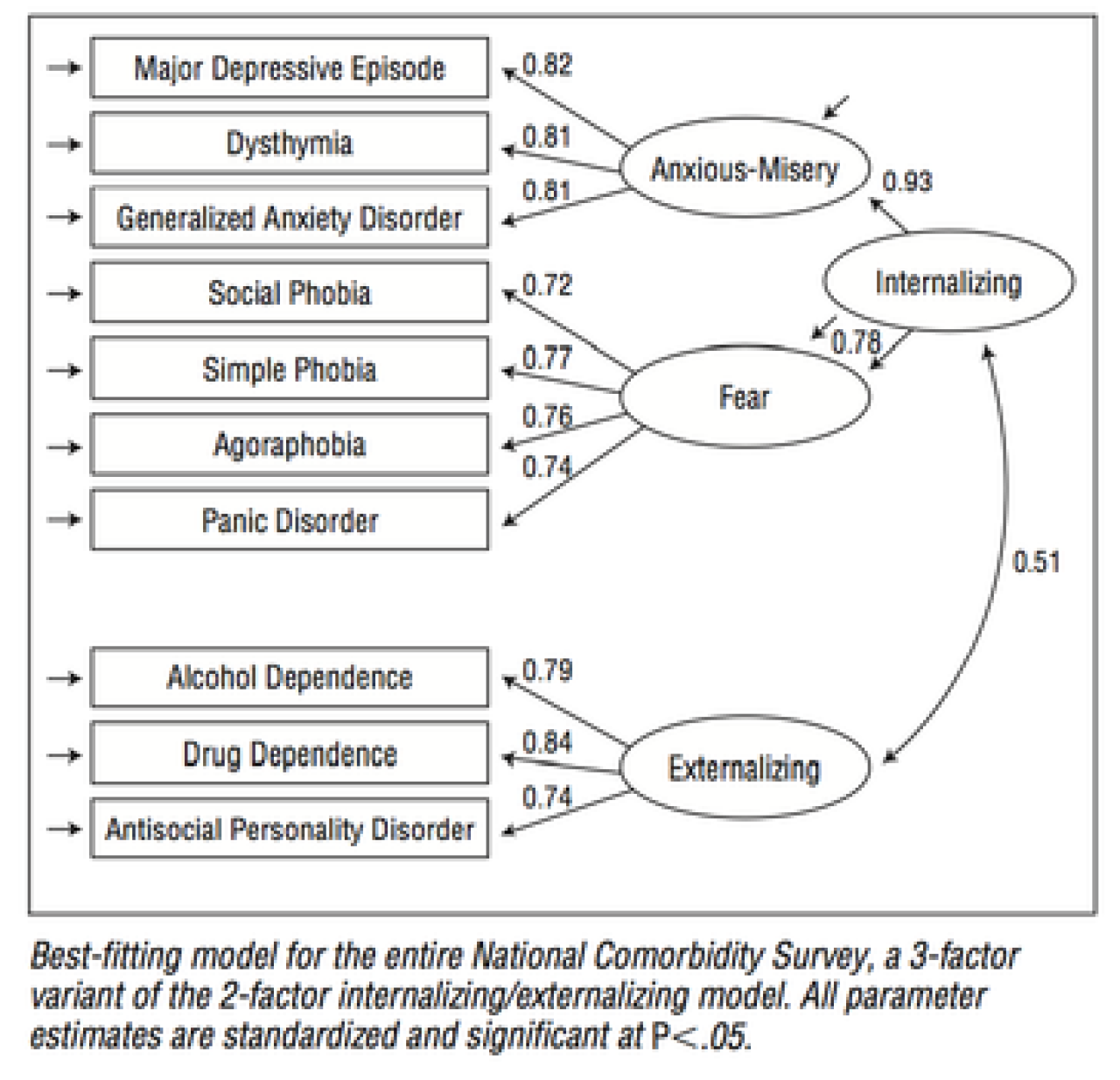
Figure 1. Example of factor structure of common psychiatric disorders. Common disorders seem to represent two latent dimensions, internalizing and externalizing disorders. From Krueger, R. F., 1999, The structure of common mental disorders. Archives of General Psychiatry. 56: 921-926.
Factor analysis was pioneered by psychologist and statistician Charles Spearman (of Spearman correlation coefficient fame) in 1904 in his work on the underlying dimensions of intelligence. Its use was hampered by onerous hand calculations until the introduction of statistical computing; since then the technique has flourished.
There are two main types of factor analysis: exploratory and confirmatory. In exploratory factor analysis (EFA, the focus of this resource page), each observed variable is potentially a measure of every factor, and the goal is to determine relationships (between observed variables and factors) are strongest. In confirmatory factor analysis (CFA), a simple factor structure is posited, each variable can be a measure of only one factor, and the correlation structure of the data is tested against the hypothesized structure via goodness of fit tests. Figure 2 is a graphic representation of EFA and CFA.

Figure 2. EFA (left) and CFA (right). Adapted from Wall, M., September 20, 2012, Session 3 guest lecture in Epidemiology of Drug and Alcohol Problems, Hassin, D., Columbia University Mailman School of Public Health
There are different factor analytic techniques for different measurement and data scenarios:
-
Observed variables are continuous, latent variables are hypothesized to be continuous
-
Observed are continuous, latent are categorical
-
Observed are categorical, latent are continuous
-
Observed are categorical, latent are categorical
This resource page will focus on scenarios 1 and 3.
Figures 3 and 4 below illustrate some basic premises of measurement theory vis-à-vis factor analysis:
-
Factors, or latent variables, systematically influence observed variables (i.e., when we measure observed variables, those measurements/observations are caused, at least in part, by latent variables)
-
Inter-individual differences (i.e., variance) in observed variables are due to latent variables and measurement error
-
Each type of factor (common, specific – see below) in addition to measurement error contributes to a portion of variance
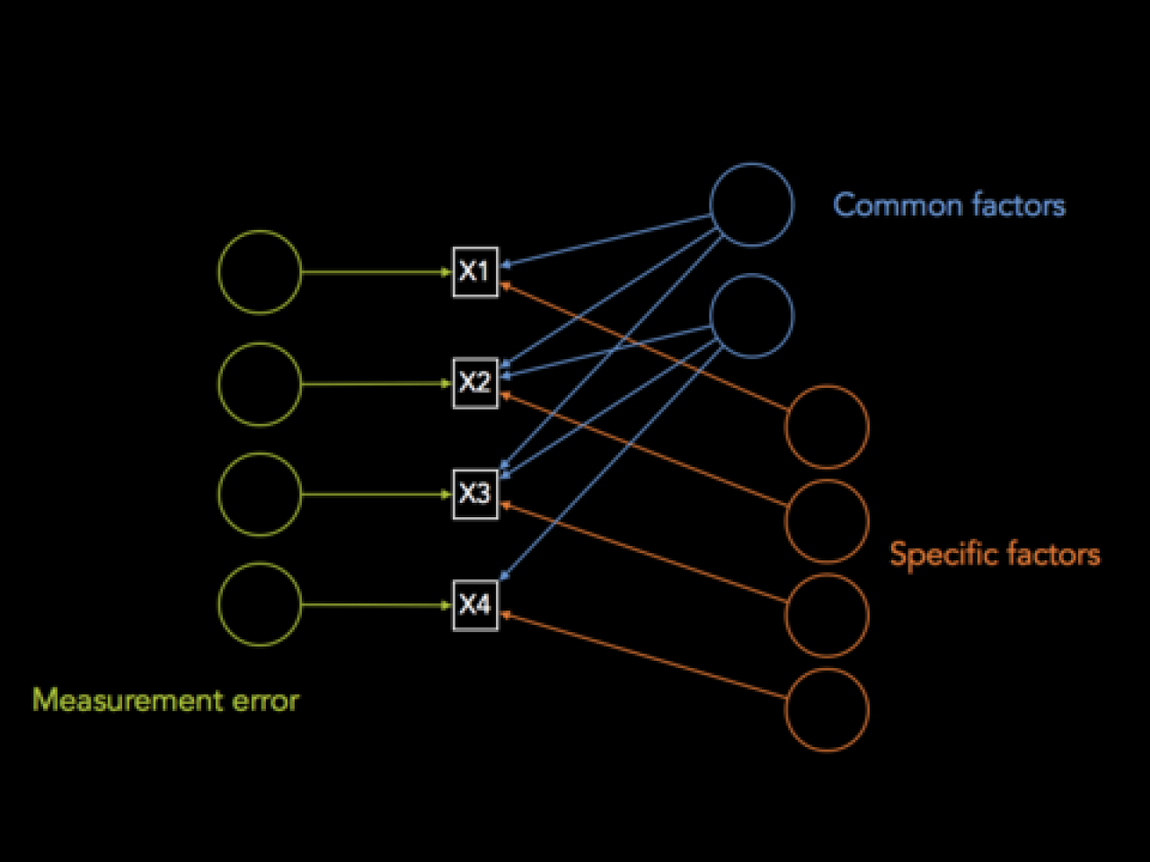
Figure 3. Elements that influence observed variables. Figure adapted from Tucker, LR and MacCallum, RC. 1997, Exploratory Factor Analysis: http://www.unc.edu/~rcm/book/factornew.htm
Figure 3 shows that three things influence observed variables. Two are types of latent variables or factors. The first are common factors, which give rise to more than one of the observed variables (e.g., “math ability” might give rise to “addition test score,” “multiplication test score,” and “division test score”). The second are specific factors, which give rise to only one of the observed variables (a common factor can become a specific factor if you remove all but one of the observed variables to which they give rise). The third thing that influences observed variables is measurement error, which is not latent, but is often due to unsystematic events that influence measurement. Measurement error is closely tied to reliability.
Each of the elements that influence observed variables also contribute to those variables’ variance. Figure 4 shows that the variance of a given observed variable is due in part to factors that influence other observed variables, factors that influence only the given observed variable, and measurement error. Common variance is sometimes referred to as “communality,” and the specific variance and error variance are often combined and referred to as “uniqueness.”
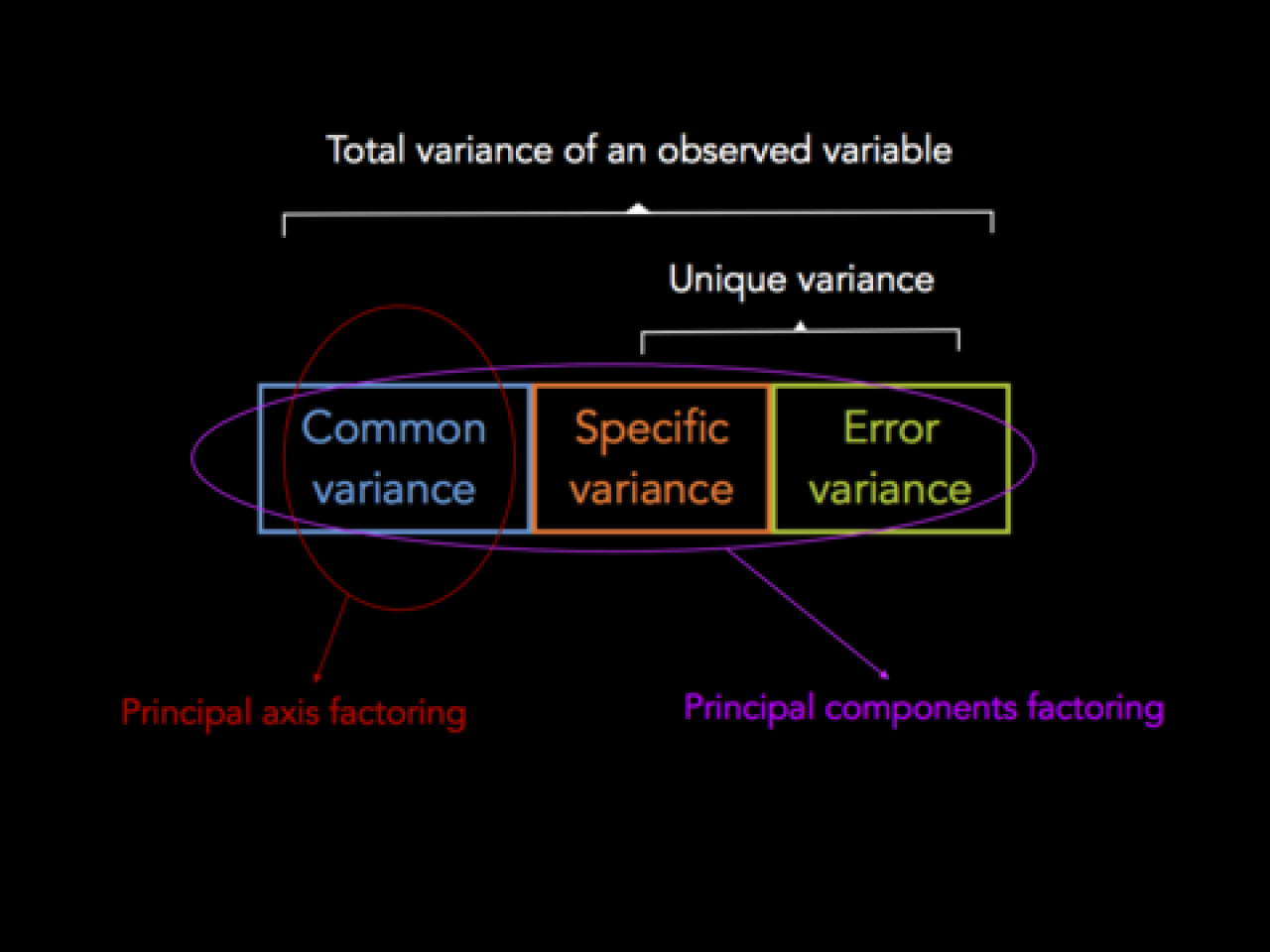
Figure 4. Variance structure of observed variables. Figure from James Neill, 2013, Exploratory Factor Analysis, Lecture 5, Survey Research and Design in Psychology. http://www.slideshare.net/jtneill/exploratory-factor-analysis
The figure also shows one key difference between factor analysis and principal components analysis. In principal components analysis, the goal is to account for as much of the total variance in the observed variables as possible; linear combinations of observed variables are used to create components. In factor analysis, the goal is to explain the covariance among variables; the observed variables are defined as linear combinations of the factors.
The main point is that factor analytic theory is about accounting for the covariation between observed variables. When observed variables are correlated with each other, factor analytic theory says that the correlation is due, at least in part, to the influence of common latent variables.
Assumptions
Factor analysis has the following assumptions, which can be explored in more detail in the resources linked below:
-
Sample size (e.g., 20 observations per variable)
-
Level of measurement (e.g., the measurement/data scenarios above)
-
Normality
-
Linearity
-
Outliers (factor analysis is sensitive to outliers)
-
Factorability
Eigenvalues and Factor Loadings
[Note: this matrix algebra review can help you understand what’s going on under the hood with eigenvalues and factor loadings, but is not completely necessary for interpreting the results of factor analysis.]
Factors are extracted from correlation matrices by transforming such matrices by eigenvectors. An eigenvector of a square matrix is vector that, when premultiplied by the square matrix, yields a vector that is an integer multiple of the original vector. That integer multiple is an eigenvalue.
The eigenvalue represents the amount of variance each factor accounts for. Each extracted factor will have an eigenvalue (the integer multiple of the original vector). The first extracted factor is going to try to absorb as much of the variance as possible, so successive eigenvalues will be lower than the first. Eigenvalues over 1 are “stable.” The total of all eigenvalues is the number of observed variables in the model.
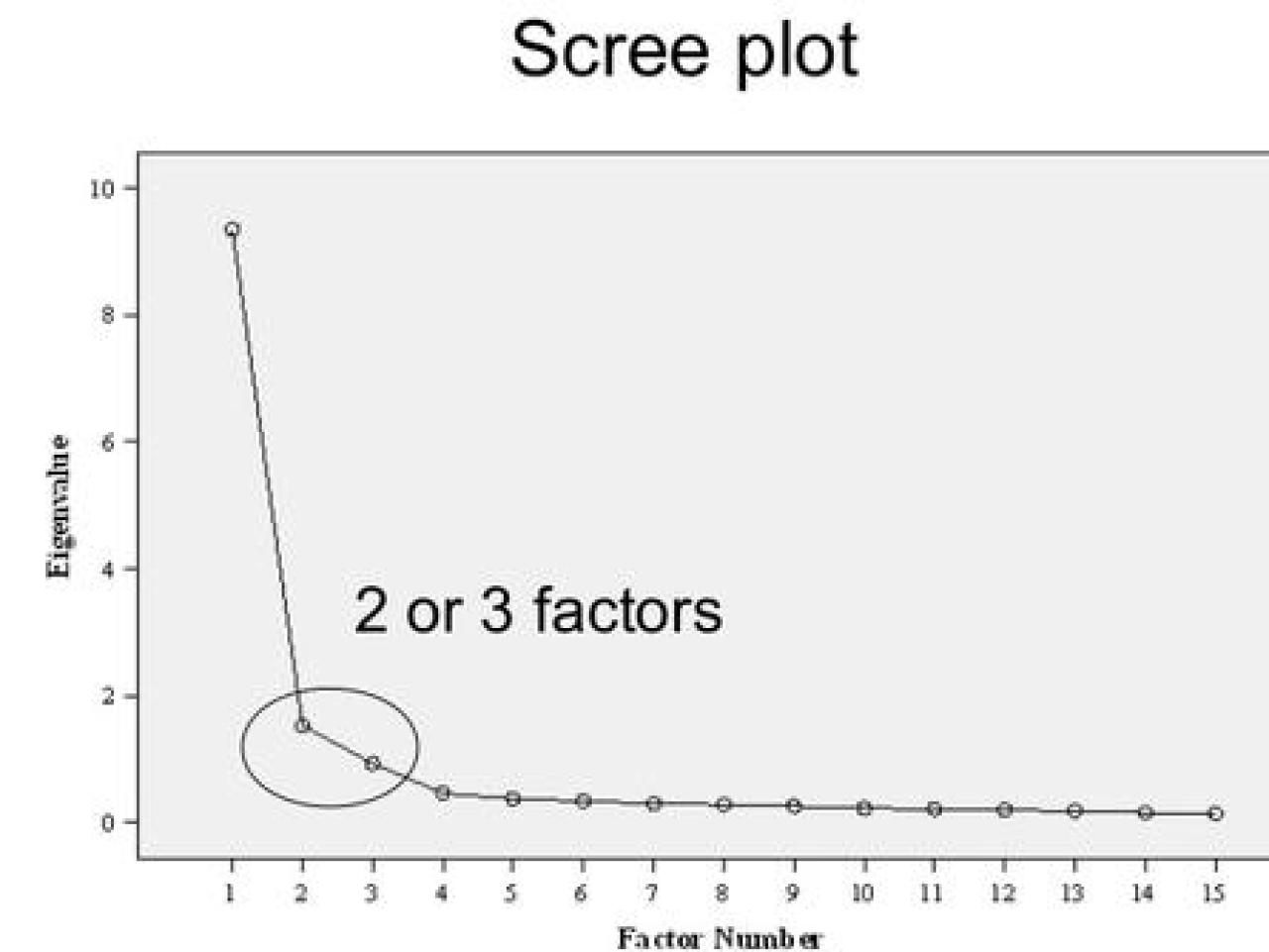
Figure 5. Scree plot, from James Neill, 2013, Exploratory Factor Analysis, Lecture 5, Survey Research and Design in Psychology. http://www.slideshare.net/jtneill/exploratory-factor-analysis
Each variable contributes a variance of 1. Eigenvalues are then allocated to factors according to amount of variance explained. Scree plots (Figure 5 below) are common output in factor analysis software, and are line graphs of eigenvalues. They depict the amount of variance explained by each factor, and the “cut off” is the number of factors right before the “bend” in the scree plot, e.g., around 2 or 3 factors in Figure 5. Eigenvalues and scree plots can guide you in determining how many factors are the best fit for your data.
Factor loadings are a matrix of how observed variables are related to the factors you’ve specified. In geometric terms, loadings are the numerical coefficients corresponding to the directional paths connecting common factors to observed variables. They provide the basis for interpreting the latent variables. Higher loadings mean that the observed variable is more strongly related to the factor. A rule of thumb is to consider loadings above 0.3.
Rotations
Factor are rotated (literally, in geometric space) in order to aid in interpretation. There are two type of rotation: orthogonal (perpendicular), in which factors are not permitted to be correlated with each other, and oblique, in which factors are free to take any position the factor space and can be correlated with each other. Examples of orthogonal rotation include varimax, quartimax, and equamax. Examples of oblique rotation include oblimin, promax, and geomin. See resources below for how to choose a rotation method.
After rotation, the factors are re-arranged to optimally go through clusters of shared variance, so the factors can be more easily interpreted. This is akin to picking a reference group in regression. Figure 6 illustrates a factor rotation using varimax, but is for conceptual purposes only. Rotations happen under the hood of your software.
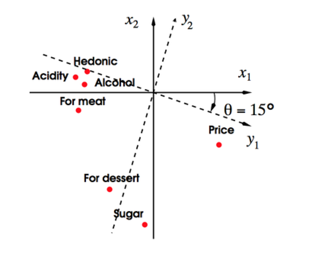
Figure 6. Example of an orthogonal varimax rotation. Observed variables were for characteristics of wine. From Abdi, Hervé. http://www.utdallas.edu/~herve/Abdi-rotations-pretty.pdf
EFA with dichotomous items
A Pearson correlation matrix is not appropriate for categorical or dichotomous items, so in order to perform EFA on such data, you need to create an appropriate correlation matrix, called tetrachoric (for dichotomous items) or polychoric (for other categorical items). A tetrachoric correlation matrix is the inferred Pearson correlation from a 2×2 table with the assumption of bivariate normality. Polychoric generalizes this to an n x m table.
The idea, illustrated by Figure 7, is that dichotomous items represent
underlying continuous constructs. In creating a tetrachoric correlation matrix, you are basically estimating a model based on proportions that fall in each area of the bottom right corner of Figure 7. The computer tries numerous thresholds and combinations.

Figure 7. Representation of observed dichotomous variable (depressed yes/no) and a continuous latent construct. The bottom corner shows how the latter is modeled by the former.
As of spring 2013, MPlus is the gold standard for conducting EFA on dichotomous items, but it is also possible to implement in R. See resources below, in particular, the “Psych” package documentation.
Readings
Textbooks & Chapters
-
Exploratory Factor Analysis: An online book manuscript by Ledyard Tucker and Robert MacCallum that provides an extensive technical treatment of the factor analysis model as well as methods for conducting exploratory factor analysis.
-
Exploratory and Confirmatory Factor Analysis: Understanding Concepts and Applications
Methodological Articles
Methodological (theory and background)
-
Exploratory Factor Analysis, Theory Generation, and Scientific Method
-
A Brief History of the Philosophical Foundations of Exploratory Factor Analysis.
Methodological (applied)
Application Articles
-
Nicotine dependence, abuse and craving: dimensionality in an Israeli sample.
-
The Senior Authors’ Response: Factor Analysis as a Tool for Evaluating Eating Patterns
Software
-
R demo code from Prins’ presentation:
install.packages(“psych”)
library(psych)
?fa
#quick demo of exploratory factor analysis
data(Harman)
head(Harman.Holzinger) # 9×9 correlation matrix of cognitive ablity tests, N=696
cor.plot(Harman.Holzinger)
pa <- fa(Harman.Holzinger, 4, fm=”pa”, rotate=”varimax”, SMC=FALSE)
#There are other factoring methods for different scenarios: minimum residual (minres), #principal axes (as above), weighted least squares, or maximum likelihood. See “arguments” #section of ?fa, and details.
print(pa, sort=TRUE)
#prints results, sort=TRUE shows loadings by absolute value. u^2 is uniqueness and h^2 is #reliability. See “values” in ?fa for how to call specific results
scree(Harman.Holzinger,factors=TRUE,pc=TRUE,main=”Scree plot”,hline=NULL,add=FALSE)
#creates a scree plot — a line graphs of eigenvalues. They depict the amount of variance #explained by each factor, and the “cut off” is the number of factors right before the “bend” #in the scree plot, e.g., around 2 or 3 factors in Figure 5. Eigenvalues and scree plots can #guide you in determining how many factors are the best fit for your data.
fa.plot(pa, labels=TRUE) #a graphic plot of factor loadings
fa.diagram(pa, sort=TRUE, cut=.3, simple=TRUE, errors=FALSE, digits=1, e.size=.05, rsize=0.15)
#a familiar-looking diagram of the relationship between factors and observed variables
#code for dichotomous items
your.data<-read.csv(“”, header=TRUE, stringsAsFactors=FALSE)
your.fa<-fa.poly(your.data, nfactors=3, n.obs = 184, n.iter=1, rotate=”geominQ”, scores=”tenBerge”, SMC=TRUE, symmetric=TRUE, warnings=TRUE, fm=”wls”,
alpha=.1, p =.05, oblique.scores=TRUE)
#the major difference here is the rotation (you need to pick an oblique method — geominQ is #closest to what MPlus does), factoring method (weighted least squares, or wls, is closest to #MPlus but not exact), and scores = “tenBerge”.
#if you want to make the tetrachoric correlation matrix yourself, use the polychor package
install.packages(“polycor”)
library(polycor)
?hetcor
Courses
-
Here at Mailman: P8158 – Latent variable and structural equation modeling for health sciences. Melanie Wall.