Competing Risk Analysis
|
Software |
|
|
Websites |
|
Overview
Competing risk analysis refers to a special type of survival analysis that aims to correctly estimate marginal probability of an event in the presence of competing events. Traditional methods to describe survival process, such Kaplan Meier product-limit method, are not designed to accommodate the competing nature of multiple causes to the same event, therefore they tend to produce inaccurate estimates when analyzing the marginal probability for cause-specific events. As an work-around, Cumulative Incidence Function (CIF) was proposed to solve this particular issue by estimating the marginal probability of a certain event as a function of its cause-specific probability and overall survival probability. This method hybridizes the idea of product-limit approach and the idea of competing causal pathways, which provides a more interpretable estimate for the survival experience of multiple competing events for a group of subjects. Like many analyses, the competing risk analysis includes a non-parametric method which involves the use of a modified Chi-squared test to compare CIF curves between groups, and a parametric approach which model the CIF based on a subdistribution hazard function.
Description
1. What is “competing event” and “competing risk”?
In standard survival data, subjects are supposed to experience only one type of event over follow-up, such as death from breast cancer. On the contrary, in real life, subjects can potentially experience more than one type of a certain event. For instance, if mortality is of research interest, then our observations – senior patients at an oncology department, could possibly die from heart attack or breast cancer, or even traffic accident. When only one of these different types of event can occur, we refers to these events as “competing events”, in a sense that they compete with each other to deliver the event of interest, and the occurrence of one type of event will prevent the occurrence of the others. As a result, we call the probability of these events as “competing risks”, in a sense that the probability of each competing event is somehow regulated by the other competing events, which has an interpretation suitable to describe the survival process determined by multiple types of events.
To better understand the competing event scenario, consider the following examples:
1) A patient can die from breast cancer or from stroke, but he cannot die from both;
2) A breast cancer patient may die after surgery before they can develop hospital infection;
3) A soldier may die during a combat or in a traffic accident.
In the examples above, there are more than one pathway that a subject can fail, but the failure, either death or infection, can only occur once for each subject (without considering recurring event). Therefore, the failures caused by different pathways are mutually exclusive and hence called competing events. Analysis of such data requires special considerations.
2. Why shouldn’t we use Kaplan Meier estimator?
Like in standard survival analysis, the analytical object for competing event data is to estimate the probability of one event among the many possible events over time, allowing the subjects to fail from competing events. In the above examples, we might want to estimate the breast cancer mortality rate over time, and want to know whether the mortality rate of breast cancer differ between two or more treatment groups, with or without adjustment of covariates. In standard survival analysis these questions can be answered by using Kaplan Meier product limit method to obtain event probability over time, and Cox proportional hazard model to predict such probability. Likewise, in competing event data, the typical approach involves the use of KM estimator to separately estimate probability for each type of event, while treating the other competing events as censored in addition to those who are censored from loss to follow-up or withdrawal. This method of estimating event probability is called cause-specific hazard function, which is mathematically expressed as:
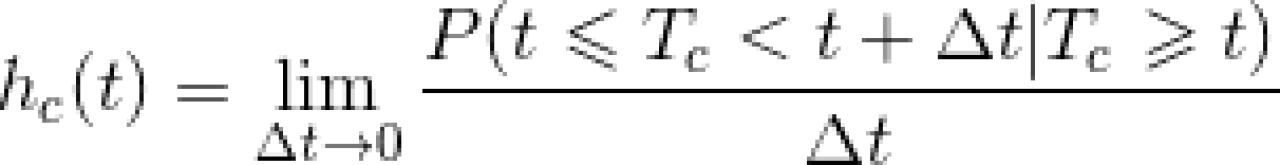
The random variable Tc denotes the time to failure from event type c, therefore the cause-specific hazard function hc(t) gives the instantaneous failure rate at time t from event type c, given not failing from event c by time t.
Correspondingly, there is a cause-specific hazard model based on the Cox proportional hazard model which has the form of:
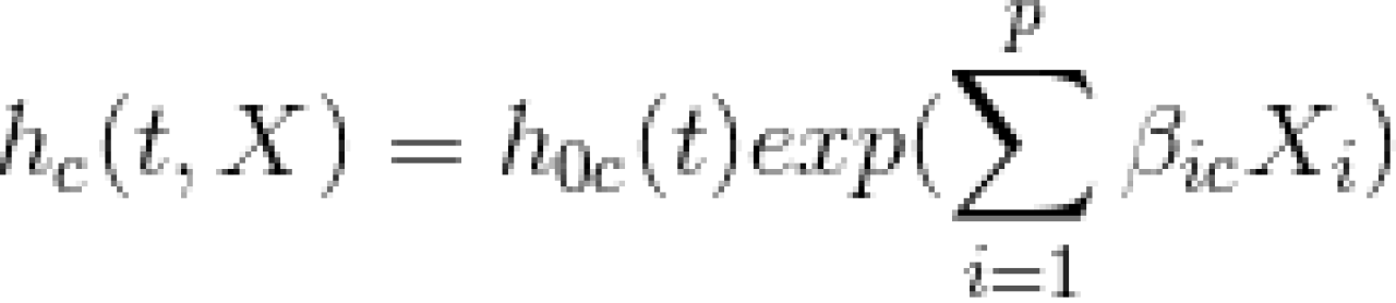
This proportional hazard model of event type c at time t allows effects of the covariates to differ by event types, as the subscripted beta coefficient suggests.
Using these methods, one can separately estimate failure rate for each one of competing events. For instance, in our breast cancer mortality example, when death from breast cancer is the event of interest, the death from heart attack and all other causes should be treated as censored in addition to conventional censored observations. This would allow us to estimate the cause-specific hazard for breast cancer mortality rate, and go on to fit a cause-specific hazard model on breast cancer mortality. The same procedure can apply to death from heart attack when it becomes event of interest.
A major caveat of the cause-specific approach is that it still assumes independent censoringfor subjects who are not actually censored but failed from competing events, as for standard censorship such as loss to follow up. Suppose this assumption is true, when focusing on cause-specific death rate from breast cancer, then any censored subject at time t would have the same death rate from breast cancer, regardless of whether the reason for censoring is either CVD or other cause of death, or loss to follow-up. This assumption is equivalent to sayingcompeting events are independent, which is the foundation for the KM type of analysis to be valid. However, there is no way to explicitly test whether this assumption is satisfied for any given dataset. For instance, we can never determine whether a subject who died from heart attack would have died from breast cancer if he did not die from heart attack, since the possible death from cancer is unobservable for subjects died from heart attack. Therefore, estimates from cause-specific hazard function do not have an informative interpretation since it relies heavily on the independence censoring assumption.
3. What’s the solution?
Up to date, the most popular alternative approach to analyze competing event data is called theCumulative Incidence Function (CIF), which estimates the marginal probability for each competing event. Marginal probability is defined as the probability of subjects who actually developed the event of interest, regardless of whether they were censored or failed from other competing events. In the simplest case, when there is only one event of interest, the CIF should equal the (1-KM) estimate. When there are competing events, however, the marginal probability of each competing events can be estimated from CIF, which is derived from the cause-specific hazard as we discussed previously. By definition, the marginal probability does not assume the independence of competing events, and it has an interpretation that is more relevant to clinician in cost-effectiveness analyses in which risk probability is used to assess treatment utility.
3.1 Cumulative Incidence Function (CIF)
The construction of a CIF is as straight forward as the KM estimate. It is a product of two estimates:
1) The estimate of hazard at ordered failure time tf for event-type of interest, expressed as:

where the mcf denotes the number of events for risk c at time tf and nf is the number of subjects at that time.
2) The estimate of overall probability of surviving previous time (td-1):

where S(t) denotes the overall survival function rather than the cause specific survival function. The reason why we have to take overall survival into consideration is simple yet important: a subject must have survived all other competing events in order to fail from event type c at timetf.
With these two estimates, we can compute the estimated incidence probability of failing from event-type c at time tf as:

The equation is self-explanatory: the probability of failing from event type c at time tf is simply the product of surviving the previous time periods and the cause specific hazard at time tf.
The CIF for event type c at time tf is then the cumulative sum up to time tf (i.e., from f’=1 to f’=f) of these incidence probabilities over all event type c failure times, which is expressed as:

As we mentioned before, the CIF is equivalent to 1-KM estimator when there is no competing event. When there is competing event, the CIF differs from 1-KM estimator in that it uses overall survival function S(t) that counts failures from competing events in addition to the event of interest, whereas the 1-KM estimator uses the event-type specific survival function Sc(t), which treats failures from competing events as censored.
By using the overall survival function, CIF bypasses the need to make unverifiable assumptions of independence of censoring on competing events. Since the S(t) is always less than Sc(t), in competing event data, the CIF is always smaller than 1-KM estimates, which means the 1-KM tends to overestimate the probability of failure from the event type of interest. Another advantage is that, by definition, the CIF of each competing event is a fraction of the S(t), therefore the sum of each individual hazard for all competing events should equal the overall hazard. This property of CIF makes it possible to dissect overall hazard, which has more practical interpretations.
3.2 Non-parametric analysis
Gray (1988) proposed a non-parametric test to compare two or more CIFs. The test is analogous to the log-rank test comparing KM curves, using a modified Chi-squared test statistic. This test does not require the independent censoring assumption. Please read the original article for details on how this test statistics is constructed.
3.3 Parametric analysis
Fine and Gray (1999) proposed a proportional hazards model aims at modeling the CIF with covariates, by treating the CIF curve as a subdistribution function. The subdistribution function is analogous to the Cox proportional hazard model, except that it models a hazard function (as known as subdistribution hazard) derived from a CIF. The Fine and Gray subdistribution hazard function for event type c can be expressed as:

The above function estimates the hazard rate for event type c at time t based on the risk set that remains at time t after accounting for all previously occurring event types, which includes competing events.
The CIF based proportional hazard model is then defined as:

This model satisfied the proportional hazard assumption for the subpopulation hazard being modeled, which means the general hazard ratio formula is essentially the same as for the Cox model, except a minor cosmetic difference that the betas in the Cox model is replaced by gammas in Fine and Gray’s model. Consequently, we should interpret the gammas in a similar way as we do for the betas estimated from a Cox model, except that it estimates the effect of certain covariates in the presence of competing events. The Fine and Gray model can also be extended to allow for time-dependent covariates.
Today, analysis of competing data using either non-parametric or parametric method is available in the major statistical packages including R, STATA and SAS.
Readings
Textbooks & Chapters
J. D. Kalbfleisch, and Ross L. Prentice, ‘Competing Risks and Multistate Models’, in The Statistical Analysis of Failure Time Data (Hoboken, N.J.: J. Wiley, 2002), pp. 247-77.
The idea of CIF was first proposed in this book. It gives you a convincing rationale as to why you can’t analyze competing data using Kaplan Meier method.
David G. Kleinbaum, and Mitchel Klein, ‘Competing Risks Survival Analysis’, in Survival Analysis : A Self-Learning Text (New York: Springer, 2012), pp. 425-95.
This entire page borrowed heavily from this awesome chapter by Kleinbaum & Klein, I highly recommend it! P.S. I highly recommend all statistical textbooks by Kleinbaum in general.
Bob Gray (2013). cmprsk: Subdistribution Analysis of Competing Risks. R package version 2.2-6. https://cran.r-project.org/web/packages/cmprsk/index.html
This is the R package “cmprsk” user manual, it provides human being friendly guidance on how to implement those functions.
“stcrreg — Competing-risks regression”, StataCorp. 2013. Stata 13 Base Reference Manual. College Station, TX: Stata Press.
This is the STATA user manual, I know very little about it but seems to be informative to skilled STATA users.
“Proportional Subdistribution Hazards Model for Competing-Risks Data”, SAS Institute Inc. 2013. SAS/STAT® 13.1 User’s Guide: pp5991-5995. Cary, NC: SAS Institute Inc.
This is one of those SAS forum papers that describes how to analyze competing risk using PROC PHREG in SAS. Very detailed and useful.
Methodological Articles
Prentice, Ross L., et al. “The analysis of failure times in the presence of competing risks.” Biometrics (1978): 541-554.
This paper is very similar to the book chapter by Kalbfleisch and Prentice, probably they are the same paper.
Gray, Robert J. “A class of K-sample tests for comparing the cumulative incidence of a competing risk.” The Annals of statistics (1988): 1141-1154.
This is the paper that proposed the modified Chi-squared test to compare two or more CIFs. Epic!
Fine, Jason P., and Robert J. Gray. “A proportional hazards model for the subdistribution of a competing risk.” Journal of the American Statistical Association 94.446 (1999): 496-509.
This is the paper that proposed the subdistribution hazard function and the proportional hazard model for CIF. Epic!
Latouche, Aurélien, et al. “Misspecified regression model for the subdistribution hazard of a competing risk.” Statistics in medicine 26.5 (2007): 965-974.
This paper criticized the misuse of subdistribution hazard function in published papers. It’s kind of helpful since it pointed out some common mistakes in using this method.
Lau, Bryan, Stephen R. Cole, and Stephen J. Gange. “Competing risk regression models for epidemiologic data.” American journal of epidemiology 170.2 (2009): 244-256.
This paper gives an excellent summary of the CIF and competing risk regression, with vivid graphs. It also has an application of this method in real world data. Very useful for epidemiologists.
Zhou, Bingqing, et al. “Competing risks regression for stratified data.” Biometrics 67.2 (2011): 661-670.
The paper extended Gray’s methods to analyze stratified data.
Zhou, Bingqing, et al. “Competing risks regression for clustered data.” Biostatistics 13.3 (2012): 371-383.
The paper extended Gray’s methods to analyze clustered data.
Andersen, Per Kragh, et al. “Competing risks in epidemiology: possibilities and pitfalls.” International journal of epidemiology 41.3 (2012): 861-870.
A good summary and critique of Gray’s methods.
Application Articles
Wolbers, Marcel, et al. “Prognostic models with competing risks: methods and application to coronary risk prediction.” Epidemiology 20.4 (2009): 555-561.
This paper compared Fine and Gray’s model to standard Cox model in analyzing coronary heart disease mortality and showed Cox model overestimated the hazard.
Wolbers, Marcel, et al. “Competing risks analyses: objectives and approaches.” European Heart Journal (2014): ehu131.
This paper is also by Wolbers et al. but gives a more extensive review of Gray’s method and an example analysis of implantable cardioverter-defibrillators effectiveness.
Grover, Gurprit, Prafulla Kumar Swain, and Vajala Ravi. “A Competing Risk Approach with Censoring to Estimate the Probability of Death of HIV/AIDS Patients on Antiretroviral Therapy in the Presence of Covariates.” Statistics Research Letters 3.1 (2014).
A classic application in HIV treatment research.
Dignam, James J., Qiang Zhang, and Masha Kocherginsky. “The use and interpretation of competing risks regression models.” Clinical Cancer Research 18.8 (2012): 2301-2308.
This paper used an example data from a radiation therapy oncology group clinical trial for prostate cancer to show that different model of hazard can lead to very different conclusions about the same predictor.
R Tutorials
Scrucca, L., A. Santucci, and F. Aversa. “Competing risk analysis using R: an easy guide for clinicians.” Bone marrow transplantation 40.4 (2007): 381-387.
A very nice tutorial of estimating CIF in R for non-statsitical people.
Scrucca, L., A. Santucci, and F. Aversa. “Regression modeling of competing risk using R: an in depth guide for clinicians.” Bone marrow transplantation 45.9 (2010): 1388-1395.
A very nice tutorial of fitting competing risk regression in R for non-statsitical people.
Scheike, Thomas H., and Mei-Jie Zhang. “Analyzing competing risk data using the R timereg package.” Journal of statistical software 38.2 (2011).
An intro to an R package “timereg” other than the “cmprsk” package for competing data analysis.
STATA tutorials
Coviello, Vincenzo, and May Boggess. “Cumulative incidence estimation in the presence of competing risks.” STATA journal 4 (2004): 103-112.
SAS tutorials
Lin, Guixian, Ying So, and Gordon Johnston. “Analyzing survival data with competing risks using SAS software.” SAS Global Forum. Vol. 2102. 2012.
Courses
Sally R. Hinchlie. “Competing Risks – What, Why, When and How?” Survival Analysis for Junior Researchers, Department of Health Sciences, University of Leicester, 2012
An awesome lecture on competing risk analysis with lots of graphs to understand the method.
Bernhard Haller. “Analysis of competing risks data and simulation of data following predened subdistribution hazards”, Research Seminar, Institut für Medizinische Statistik und Epidemiologie, Technische Universität München, 2013
Teach you how to simulate competing data, a little bit hard to follow.
Roberto G. Gutierrez. “Competing-risks regression”, 2009 Australian and New Zealand Stata Users Group Meeting. StataCorp LP, 2009
A lecture about using STATA to analyze competing risk data.