Age-Period-Cohort Analysis
|
Software |
|
|
Courses |
Overview
This page briefly describes age-period-cohort analysis and provides an annotated resource list.
Description
Age Period Cohort Effect
Age period cohort (APC) analysis plays an important role in understanding time-varying elements in epidemiology. In particular, APC analysis discerns three types of time varying phenomena: Age effects, period effects and cohort effects. (1)
Age effects are variations linked to biological and social processes of aging specific to individuals.(2) They include physiologic changes and accumulation of social experiences linked to aging, but unrelated to the time period or birth cohort to which an individual belongs. In epidemiological studies age effects are usually denoted by varying rates of diseases across age groups.
Period effects result from external factors that equally affect all age groups at a particular calendar time. It could arise from a range of environmental, social and economic factors e.g. war, famine, economic crisis. Methodological changes in outcome definitions, classifications, or method of data collection could also lead to period effects in data. (3)
Cohort effects are variations resulting from the unique experience/exposure of a group of subjects (cohort) as they move across time. The most commonly defined group in epidemiology is the birth cohort based on year of birth and it is described as difference in the risk of a health outcome based on birth year. Thus a cohort effect occurs when distributions of disease arise from an exposure affect age groups differently. In epidemiology, a cohort effect is conceptualized as an interaction or effect modification due to a period effect that is differentially experienced through age-specific exposure or susceptibility to that event or cause.(4)
In contrast to this conceptualization of cohort effect as an effect modification in epidemiology, sociological literature consider cohort effect as a structural factor representing the sum of all unique exposures experienced by the cohort from birth. In this case, age and period effect are conceived as confounders of cohort effect and APC analysis aims to disentangle the independent effect of age, period and cohort.(4) Most of the APC analysis strategies are based on the sociological model of cohort effect, conceptualize independent effect of age, period and cohort effect.
Identification problem in APC: APC analysis aims at describing and estimating the independent effect of age, period and cohort on the health outcome under study. The different strategies used aims to partition variance into the unique components attributable to age, period, and cohort effects (4). However, there is a major impediment to independently estimating age, period, and cohort effects by modeling the data which is know as the “identification problem” in APC. This is due to the exact linear dependency among age, period, and cohort: Period – Age = Cohort; that is, given the calendar year and age, one can determine the cohort (birth year) (5). The presence of perfectly collinear predictors (age, period and cohort) in a regression model will produce a singular non-identifiable design matrix, from which it is statistically impossible to estimate unique estimates for the three effects. (5)
Conventional solutions to APC identification problem
Constrained Coefficients GLIM estimator (CGLIM)
A popular approach to resolving the identification problem was by using constraint based regression analysis (Constrained Coefficients GLIM estimator (CGLIM)). In this strategy additional constrains are placed on one of the categories of at least one predictor to simultaneously estimate the age period and cohort effect. Thus assuming some categories of age groups, cohorts or time periods have identical effects on the dependent variable it becomes possible to estimate independent effect of age period and cohort (6). However, the results from this analysis will depend on constrains chosen by the investigator based on external information. The validity of the constraints chosen will depend on the theoretical preconception about the categories of parameter that are identical, is often subjective and there is no empirical way to confirm the validity of the chosen constraints (4).
Proxy variables approach
Use one or more proxy variables as surrogates for the age, period, or cohort coefficients (7)
Nonlinear parametric (algebraic) transformation approach
Define a nonlinear parametric function of one of the age, period, or cohort variables so that its relationship to others is nonlinear.
Intrinsic estimator method
Is a new technique developed over the last 10 years and it is related to principal component analysis that addresses identification problem when explanatory variables are highly correlated. Though IE also imposes constraint on parameters similar to CGLM, the constraint are less subjective and doesn’t affect the estimation of regression parameters for age, period or cohort (4,5). Model validation studies have confirmed the robustness of the statistical properties of IE by comparing findings from an IE analysis of empirical data with results from an analysis of the same data by a different family of models that do not use the same identifying constraint (5).
Median Polish Analysis
The epidemiological definition of a cohort effect as an age by period interaction is basis for median polish analysis. It extracts the non-linearity in age and period effects and partition the non-linear variance into cohort effect and random error (4). In other words this approach evaluates the age and period interaction that is beyond what would be expected of their additive influences.
Guideline for estimating APC models (Based on Yang and Land) (5):
-
Descriptive data analysis by graphical representation of data is the first step in an APC analysis. This helps in qualitative assessment of patterns of time-based variations
-
Rule out that data can be explained by any single factor or two factor model of age, time period and cohort. A Goodness-of-fit statistics is often used to compare between reduced log linear models: three separate models for age, period and cohort effects; and three two-factor models, one for each of three possible pairs of effects, namely, AP, AC, and PC effects models. All of these models then are compared with a full APC model where all three factors are simultaneously controlled.Two most commonly used penalized-likelihood model selection criteria namely, the Akaike information criterion (AIC) and the Bayesian information criterion (BIC), are used to evaluate the model since likelihood ratio tests tend to favor models with a larger number of parameters. BIC and AIC both adjust the impact of model dimensions on model deviances.
-
If the descriptive analyses indicate that all three of the A, P, and C dimensions is not operative, then the analysis can be completed with a reduced model that omits the non-operative dimension and there is no identification problem.
-
If, however, these analyses suggest that all three dimensions are at work use one of the specific methods of APC analysis
Median Polish Analysis-Practical Example (3)
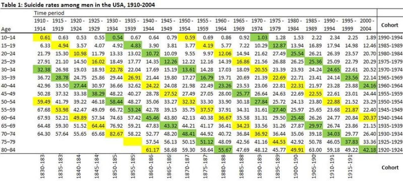
Table (3) demonstrates the identification problem, where the three components (age, period and cohort) are perfectly correlated. To identify the cohorts we need to know only the period and age group: we subtract the early age group from the upper and lower period limit (e.g. people who were 10-14 years old in 1950-1954 we subtract 10 from 1950 and 1954 to label the cohort interval as 1940-1944). (9) The color highlighted diagonal fields indicate the rate for each cohort as they age. Contingency tables cannot estimate mutually exclusive cohort risk because of overlapping cohorts. This convention may introduce misclassification of some individuals, but the primary purpose of an age-period-cohort analysis is to estimate general trends in cohort specific rather than a precise quantification of a “true” causal risk. The overlapping cohort remind us against over interpretation of estimates. We also are limited by missing data. For example we only have one point of data for the youngest group population (those aged 10-14 in 2000-2004). Using this table, we can perform an initial graphical representation with a line graph in Microsoft Excel.
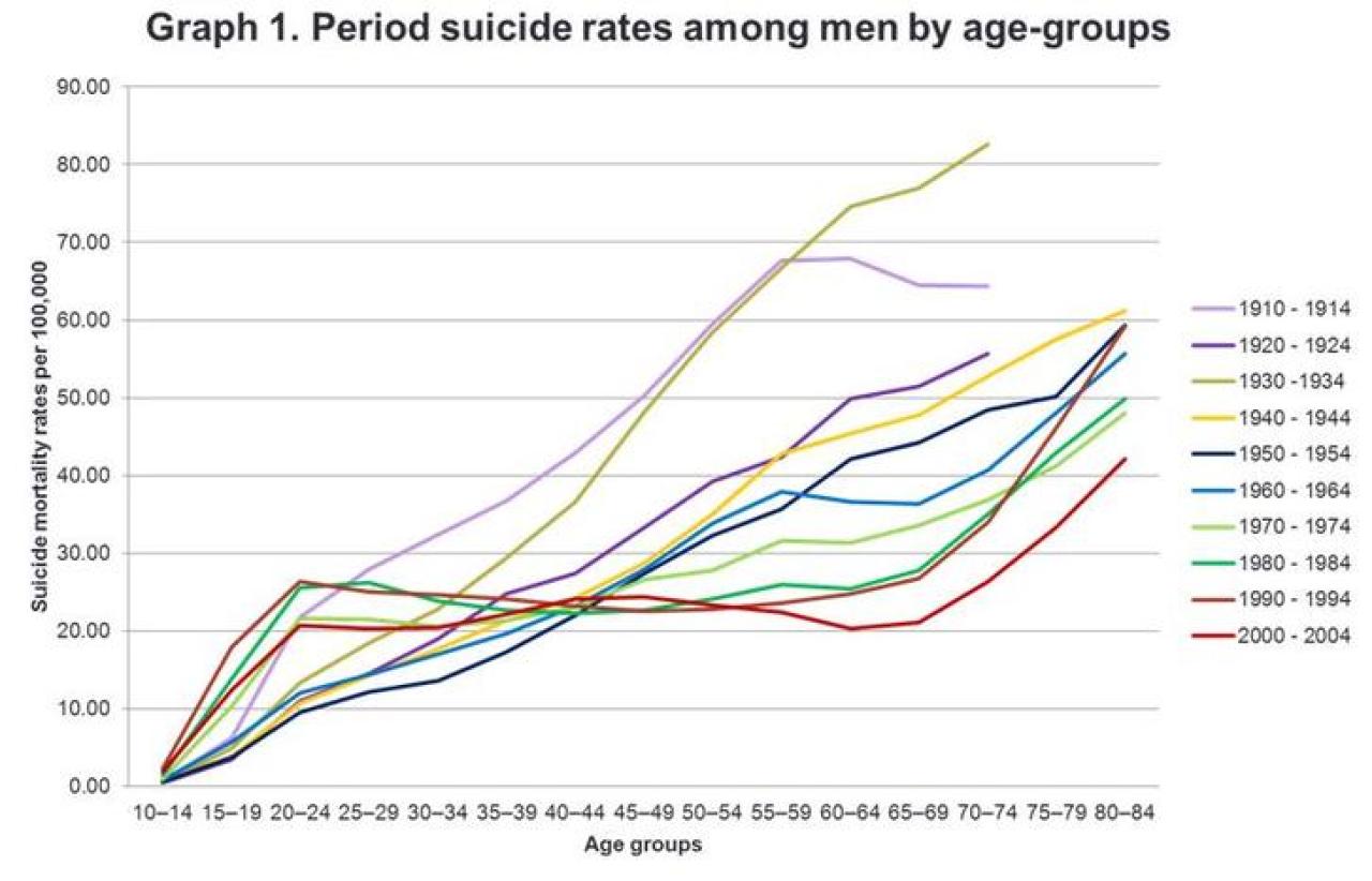
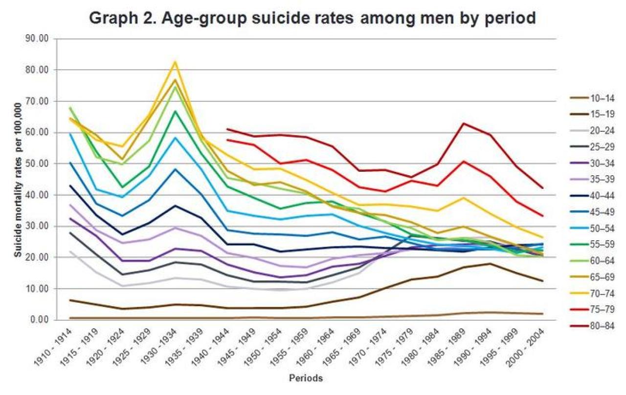
The two graphs were created using the line charts in Microsoft Excel. To plot both graphs we just rearranged the data with the “Switch Row/Column” function. These two graphical representation allow us to assessed for any pattern in the data. The limitation is that any finding could represent a mix of two or more effects.
Median polish removes the additive effects of age and period by iteratively subtracting the median value of each row and column. (6) The first step in the median polish is to calculate medians for each row, see table 2:
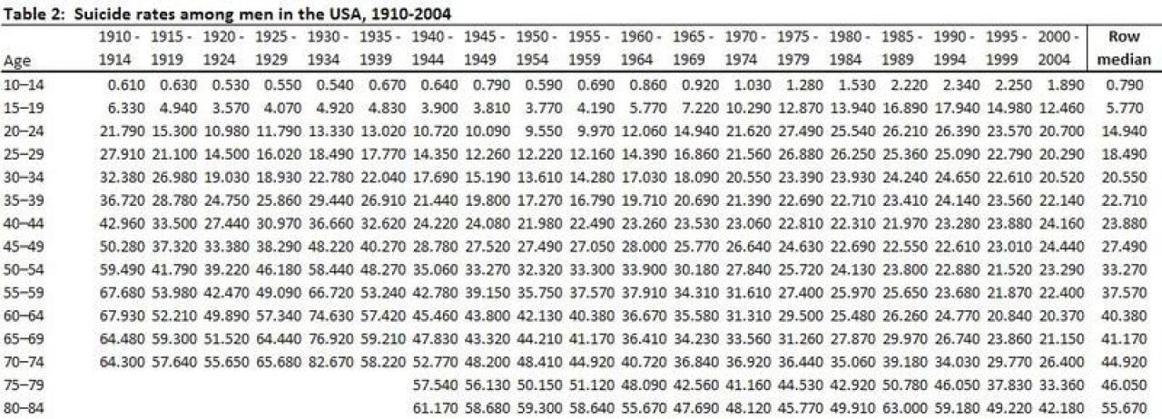
The next step is to subtract the row median from each value in the row, for example in row one we will subtract 0.610 minus 0.790 = -0.18. In the second row (15-19 years old) we used the same procedure 6.330 – 5.770 = 0.56,and then for each cell in the table. This created a table with new values, see table 3:

The next step is to calculate the column median for the new values, and then subtract the column median from each cell in the column, for example -0.18 – 19.08 = -19.26. After creating the new table with the values from subtracting each median column for each cell, we proceed to calculate the row median (third iteration). These iterations will eventually produce row and column medians equal to zero. For this example, 6 iterations were necessary to produce row and column medians equal to zero, see table 4:

Table 4 has the residuals values after 5 iterations.These residuals represent the coefficients free of the additive effect of age and period effects. Notice the data for age groups 75-79 and 80-84 years old between 1910 and 1939 are missing values. If we replace the missing values for zero rates, the calculate residuals will be biased. The full procedure was performed in Microsoft Excel. To check whether these residuals were correct, we created a new table with the product of subtracting the residual value from the original the set of values in table 1. The product of the subtractions are use to create a line chart. This line chart allow us to check the validity of the residuals and we expect lines perfectly parallel. Since we are subtracting the residuals that represent cohort effects from the original values we are assessing for any age or period effect free of cohort effects. See graphs 3 and 4:


The median polish procedure is available in R, which is a free available software (8). See the next syntax:
mpdata <- read.csv(“C:/Users/mydocs/suicidemp.csv”, header=FALSE, stringsAsFactors=FALSE)
mpdata
rownames(mpdata)<- c(“10-14”, “15-19”, “20-24”, “25-29”, “30-34”, “35-39”, “40-44”, “45-49”, “50-54”, “55-59”, “60-64”, “65-69”, “70-74”, “75-79”, “80-84”)
colnames(mpdata)<- c(“1910-1914”, “1915-1919”, “1920-1924”, “1925-1929”, “1930-1934”, “1935-1939”, “1940-1944”, “1945-1949”, “1950-1954”, “1955-1959”, “1960-1964”, “1965-1969”, “1970-1974”, “1975-1979”, “1980-1984”, “1985-1989”, “1990-1994”, “1995-1999”, “2000-2004”)
mpdata
med.p <- medpolish(mpdata, na.rm = TRUE)
med.p
Median polish results can be obtain without any transformation of rates, but using the log transformation of the rates before the median polish procedure will produce an assessment of interaction on the multiplicative scale (or log-additive effect). We repeated our median polish procedure using log transformation of the suicide rates. To produce log transformed residuals of the original table using R software we created a new function replacing the rates for log transformed rates (noticed the bold font in the syntax):
medpolish2 <- function (x, eps = 0.01, maxiter = 10L, trace.iter = TRUE, na.rm = FALSE)
{
z <- as.matrix(log(x))
nr <- nrow(z)
nc <- ncol(z)
t <- 0
r <- numeric(nr)
c <- numeric(nc)
oldsum <- 0
for (iter in 1L:maxiter) {
rdelta <- apply(z, 1L, median, na.rm = na.rm)
z <- z – matrix(rdelta, nrow = nr, ncol = nc)
r <- r + rdelta
delta <- median(c, na.rm = na.rm)
c <- c – delta
t <- t + delta
cdelta <- apply(z, 2L, median, na.rm = na.rm)
z <- z – matrix(cdelta, nrow = nr, ncol = nc, byrow = TRUE)
c <- c + cdelta
delta <- median(r, na.rm = na.rm)
r <- r – delta
t <- t + delta
newsum <- sum(abs(z), na.rm = na.rm)
converged <- newsum == 0 || abs(newsum – oldsum) < eps * newsum
if (converged)
break
oldsum <- newsum
if (trace.iter)
cat(iter, “: “, newsum, “\n”, sep = “”)
}
if (converged) {
if (trace.iter)
cat(“Final: “, newsum, “\n”, sep = “”)
}
else warning(sprintf(ngettext(maxiter, “medpolish() did not converge in %d iteration”, “medpolish() did not converge in %d iterations”), maxiter), domain = NA)
names(r) <- rownames(z)
names(c) <- colnames(z)
ans <- list(overall = t, row = r, col = c, residuals = z, name = deparse(substitute(x)))
class(ans) <- “medpolish”
ans
}
med.p2 <- medpolish2(mpdata, na.rm = TRUE)
The data is saved as a comma delimited file (.csv), an easy format to read in R. Notice the command for the median polish, the option of missing data is enable, otherwise the procedure will report an error. Both sets of residuals created with Excel and R are equal.
We reshaped the data by cohort and performed a plot of the residuals against cohort category. See next table:

We calculated the mean for each cohort and then these log transformed residuals are use to create a plot by cohort. This plot helps to assess the distribution of the residuals, where any significant deviation from zero will suggest a strong cohort effect for that cohort, see next graph:

STATA code for plotting of the residuals:
Plot of rate median polish residuals, BOOK EXAMPLE (log scale)
use “C:\Users\mydocs\suicide_data.dta”, clear
rename var2 var1
……
rename var16 var15
egen mean = rowmean( var*)
reshape long var, i(cohort) j(count)
drop if var==.
label define cohort 1 “1830-1834” 2 “1835-1839” … 32 “1985-1989” 33 “1990-1994”
label values cohort cohort
rename var Residual
twoway(scatter Residual cohort, msize(vsmall)) (connected mean cohort, msize(vsmall) msymbol(triangle) lwidth(thin) lpattern(solid)), ytitle(Median Polish Residuals) yscale (range(-2 2)) ylabel(#7) xtitle(Cohort) xlabel(#33, labels labsize(small) angle(vertical) labgap(minuscule) valuelabel) title(, size(medsmall) ring(0)) legend(size(small))
These residuals helps us to assess the magnitude of the cohort effect using a linear regression of the residuals values by cohort. Here we choose the 1910 – 1914 as the reference cohort. Similar to the graph 6, it seems that the cohorts born after 1950 were at statistical significant higher risk for suicide compared to the cohort of 1910-1014. The coefficients calculated with the linear regression are in log scale, to estimate the rate ratios we used the exponent function for each coefficient [exp(x)].

STATA code for the regression of suicide rate residuals.
char cohort[omit] 17
xi: regress Residual i.cohort
-
Yang Y, Schulhofer‐Wohl S, Fu WJ, Land KC. The Intrinsic Estimator for Age‐Period‐Cohort Analysis: What It Is and How to Use It1. American Journal of Sociology 2008;113(6):1697-736.
-
Reither EN, Hauser RM, Yang Y. Do birth cohorts matter? Age-period-cohort analyses of the obesity epidemic in the United States. Social science & medicine 2009;69(10):1439-48.
-
Keyes KM, Li G. Age–Period–Cohort Modeling. Injury Research: Springer, 2012:409-26.
-
Keyes KM, Utz RL, Robinson W, Li G. What is a cohort effect? Comparison of three statistical methods for modeling cohort effects in obesity prevalence in the United States, 1971-2006. Soc Sci Med 2010;70(7):1100-8
-
Yang, Yang, and Kenneth C. Land. Age-period-cohort analysis: new models, methods, and empirical applications. CRC Press, 2013
-
Mason, Karen Oppenheim, et al. “Some methodological issues in cohort analysis of archival data.” American sociological review (1973): 242-258
-
O’Brien, R.M. 2000. “Age Period Cohort Characteristic Models.” Social Science Research 29:123-139
-
Keyes KM, Li G. A Multiphase method for estimating cohort effects in age-period contingency table data. Ann Epidemiol 2010; 20:779-785.
Readings
Textbooks and Chapters
-
Yang, Yang, and Kenneth C. Land. Age-period-cohort analysis: new models, methods, and empirical applications. CRC Press, 2013.
-
Keyes, Katherine M., and Guohua Li. “Age–Period–Cohort Modeling.” Injury Research. Springer US, 2012. 409-426.
-
Glenn, Norval D., ed. Cohort analysis. Vol. 5. Sage, 2005
-
Hobcraft, John, Jane Menken, and Samuel Preston. Age, period, and cohort effects in demography: a review. Springer New York, 1985.
Methodological Articles
-
Ryder, Norman B. “The cohort as a concept in the study of social change.”American sociological review (1965): 843-861
-
Mason, Karen Oppenheim, et al. “Some methodological issues in cohort analysis of archival data.” American sociological review (1973): 242-258
-
Mason, William M., and Stephen E. Fienberg. “Cohort analysis in social research: beyond the identification problem.” (1985)
-
Yang, Yang, et al. “The Intrinsic Estimator for Age‐Period‐Cohort Analysis: What It Is and How to Use It1.” American Journal of Sociology 113.6 (2008): 1697-1736.
-
Keyes, Katherine M., et al. “What is a cohort effect? Comparison of three statistical methods for modeling cohort effects in obesity prevalence in the United States, 1971–2006.” Social science & medicine 70.7 (2010): 1100-1108.
-
Keyes, K. & Li, G., Age-period-cohort modeling. In Li, G. & Baker, S. (eds.),Injury Research: Theories, Methods, and Approaches. Springer, Chapter 22, pages 409-426. New York, 2012
Application Articles
-
Keyes, Katherine M., et al. “Age, Period, and Cohort Effects in Psychological Distress in the United States and Canada.” American journal of epidemiology(2014): kwu029.